


 Abstract
 HTML
HTML Reference
 Related
 PDF
PDF


-
After the discovery of the Higgs boson, continuous improvement of the sensitivity of experiments at the Large Hadron Collider (LHC) demands theoretical predictions with high order corrections. However, high order corrections could be very challenging due to the complicated multi-loop Feynman diagrams. One of the challenging tasks is to reduce the loop amplitude into a linear combination of master integrals.
For the one-loop amplitude, a variety of reduction methods has been developed [1–10]. The amplitude can be efficiently expressed as a linear combination of one-loop master integrals. After decades of effort, the one-loop reduction can now be carried out with various automated programs [11–18].
At the multi-loop level, the reduction procedure is much harder than for the one-loop case. To improve the efficiency, the reduction of the multi-loop amplitude is conventionally separated into two steps, i.e. the tensor reduction and the reduction of the scalar integrals using integration by parts (IBP). For the IBP reduction, many algorithms and codes have been developed [19–38]. On the other hand, tensor reduction is also important, and during the past decades many algorithms for tensor reduction have been proposed [39–47]. For some complicated processes, such as the full next-to-next-to-leading order QCD correction of the single-top production [48], the increasing number of form factors makes the coefficients difficult to obtain. For the two-loop five-gluon or six-gluon amplitude, the system of equations for the coefficients can be very complicated [49, 50]. Moreover, in some complicated processes, e.g.
$ e^{+}e^{-}\rightarrow Z^{\star}\rightarrow t\bar{t} $ , serious problems during tensor reduction can appear, indicating that further investigation of tensor reduction is still needed.The projection method [39, 40] is one of the most popular approaches for tensor reduction. Many important studies have been performed using this method, such as the high order QCD corrections of the Higgs production [51–54] and vector boson production [55, 56]. However, for some processes containing a fermion chain with two massive spinors, the projection method could be problematic due to the inconsistency between helicity and chirality, as is explicitly shown in next Section.
In this paper, based on the massive spinor decomposition [57–59], we propose to extend the projection method for the reduction of the loop amplitude for any process including the production of massive fermions. The massive spinor can be decomposed by defining a “null spinor” and a “reference spinor”, which have completely different equations-of-motion and polarization summation than the regular spinor. As a result, the projection method can be used for processes containing massive spinors.
The paper is organized as follows. In Section 2, we briefly review the standard projection method and demonstrate the problems due to the lack of a massless spinor. In Section 3, based on the massive spinor decomposition, we introduce the “null spinor” and the “reference spinor”, which can be used to extend the projection method for all processes. In Sections 4 and 5, we take the one-loop and two-loop diagrams for a virtual Z boson decaying into a top-quark pair to demonstrate the effectiveness of our approach. The conclusions are presented in the last section.
-
In the projection method, the loop amplitude can be expressed as a linear combination of several monomials. In each monomial the Lorentz structure is composed of the spinors and polarization vectors associated with the contracted momenta, while the remanent factors which include the coupling constants and scalar products of momenta do not affect the tensor reduction. By suppressing the spinor chirality from the Lorentz structure, we can obtain the primitive amplitude. Therefore, the loop amplitude can be decomposed as
$ {\cal A} = \sum\limits_{p,X} C_{p,X} {\cal M}_{p,X}, $

(1) where
$ X $ is the chirality index and$ p $ indicates the different primitive amplitudes.$ {\cal M}_{p,X} $ is the Lorentz structure for the chirality$ X $ and$ C_{p,X} $ is the relevant coefficient.For convenience, we can define a map for each primitive amplitude from the helicity state
$ H $ to chirality state$ X $ $ f_p: H \mapsto X, {\; s.t.\; } {\mathbb P}_H {\cal M}_{p,X} \neq 0, $

(2) where
$ {\mathbb P}_H $ is the helicity projection operator. For instance, the explicit map for the primitive amplitude$ \bar u(k_1) {\not\!\! q} v(k_2), $

(3) where
$ k_1^2 = k_2^2 = 0 $ , can be written as$ f_p(+-) = LR, \quad f_p(-+) = RL. $

(4) Furthermore, for the primitive amplitude with one massive spinor, for example
$ \bar u(k_1) {\not\!\! q} v(k_2), $

(5) where
$ k_1^2\neq0 $ and$ k_2^2 = 0 $ , the map can be constructed as$ f_p(--) = f_p(+-) = LR, \quad f_p(++) = f_p(-+) = RL. $

(6) Obviously, the map is based on at least one massless spinor, which has an equivalence relation between helicity and chirality, and can be used to fix the chirality of the relevant fermion chain by using the anti-commuting
$ \gamma_5 $ scheme. However, the map does not exist for the primitive amplitude containing two massive spinors in the same fermion chain, which is the case for which the projection method fails.Therefore we can obtain
$ {\cal M}_{p,X} = \sum\limits_H {\mathbb P}_H {\cal M}_{p,X} = \sum\limits_{H = f_p^{-1}(X)} \delta_{X,f_p(H)}{\cal M}_{p,H}, $

(7) where
$ H $ indicates the helicity state of the spinors.$ f_p^{-1}(X) $ is not the inverse of$ f_p $ but represents the set of helicity states that can be mapped to the chirality state$ X $ .Consequently, the amplitude
$ {\cal A} $ can be expressed as a linear combination of helicity primitive amplitudes,$ {\cal A} = \sum\limits_{p,H}C_{p,X = f(H)} ( {\mathbb P}_H {\cal M}_{p} ). $

(8) Now, one only needs the tensor reduction of the primitive amplitude
$ {\cal M}_p $ , so that the loop amplitude$ {\cal A} $ can be reconstructed by applying the helicity projection$ {\mathbb P}_H $ and summing all primitive amplitude choices$ p $ and helicity states$ H $ . The above derivation also gives the formula for the helicity amplitude$ {\cal A}_H = \sum\limits_{p}C_{p,X = f(H)} ( {\mathbb P}_H {\cal M}_{p} ). $

(9) In order to perform the tensor reduction of the primitive amplitude
$ {\cal M}_p $ , one needs to find a complete set of linearly independent form factors$ \{F_i\} $ .$ {\cal M}_p $ can then be projected on the form factors$ {\cal M}_p = \sum\limits_{i} d_{i,p} F_i. $

(10) To obtain an explicit expression of the coefficient
$ d_{i,p} $ , both sides of Eq. (10) are multiplied by the conjugate form factor$ F^\dagger_j $ . The form factor matrix is then defined as$ M_{ij}\equiv F_iF_j^\dagger. $

(11) The coefficient
$ d_{i,p} $ can be obtained by inversion of the matrix$ M $ $ d_{i,p} = \sum\limits_{j} (M^{-1})_{ij}{\cal M}_p F_j^\dagger. $

(12) Finally, the amplitude
$ {\cal A} $ can be expressed as a linear combination of$ {\mathbb P}_{H} F_i $ $ {\cal A} = \sum\limits_{i,H} c_{i,H}({\mathbb P}_{H} F_i), $

(13) where
$ c_{i,H} = \sum\limits_{p}d_{i,p}C_{p,X = f(H)}. $

(14) Here,
$ {\mathbb P}_{H} F_i $ is independent of the loop momenta, and can be further expressed in spinor representation. The coefficients$ c_{i,H} $ contain scalar integrals, which can be further reduced by the IBP method. -
In the previous Section, it was seen that the problem of the projection method is the lack of a massless spinor. One of the convenient approaches is to decompose the massive momentum
$ k $ by introducing the reference momentum$ k_r $ [57–59],$ k = k_0+\dfrac{m^2_k}{2 k_{0}\cdot k_{r}}k_{r}, $

(15) where
$ k^2_{0} = k^2_{r} = 0 $ and$ k^2 = m^2_k $ . The massive spinor can be decomposed as$ \begin{split} u^+(k,m_k)& = \left|k_{0} \right \rangle+\dfrac{m_k}{\left[k_{0}k_{r}\right]}\left|k_{r}\right],\\ u^-(k,m_k)& = \left|k_{0} \right ]+\dfrac{m_k}{\left\langle k_{0}k_{r}\right\rangle}\left|k_{r}\right\rangle,\\ v^+(k,m_k)& = \left|k_{0} \right ]-\dfrac{m_k}{\left\langle k_{0}k_{r}\right\rangle}\left|k_{r}\right\rangle,\\ v^-(k,m_k)& = \left|k_{0} \right \rangle-\dfrac{m_k}{\left[k_{0}k_{r}\right]}\left|k_{r}\right]. \end{split} $

(16) The two terms on the right-hand side of the above equations can be defined as two special spinors, so that
$ \begin{split} u(k,m_k)& = u_{0}(k_0)+ u_{r}(k_{r}),\\ v(k,m_k)& = v_{0}(k_0)+ v_{r}(k_{r}). \end{split} $

(17) Explicitly
$ \begin{split} u^+_{0}(k_0) &\equiv \left|k_{0} \right \rangle,\quad u^+_{r}(k_{r}) \equiv \dfrac{m_k}{\left[k_{0}k_{r}\right]}\left|k_{r}\right],\\ u^-_{0}(k_0) &\equiv \left|k_{0} \right ],\quad u^-_{r}(k_{r}) \equiv \dfrac{m_k}{\left\langle k_{0}k_{r}\right\rangle}\left|k_{r}\right\rangle,\\ v^+_{0}(k_0) &\equiv \left|k_{0} \right ],\quad v^+_{r}(k_{r}) \equiv -\dfrac{m_k}{\left\langle k_{0}k_{r}\right\rangle}\left|k_{r}\right\rangle,\\ v^-_{0}(k_0) &\equiv \left|k_{0} \right \rangle,\quad v^-_{r}(k_{r}) \equiv -\dfrac{m_k}{\left[k_{0}k_{r}\right]}\left|k_{r}\right]. \end{split} $

(18) We now define
$ u_r $ and$ v_r $ as the “reference spinors”, although they are not orthogonal to the “null spinors”$ u_0 $ and$ v_0 $ . The polarization summation formula can be written as$ \begin{split} u^+_{0}(k_0) \bar{u}^+_{0}(k_0) + u^-_{0}(k_0) \bar{u}^-_{0}(k_0) & = {{\not\! k}_0},\\ v^+_{0}(k_0) \bar{v}^+_{0}(k_0) + v^-_{0}(k_0) \bar{v}^-_{0}(k_0) & = {{\not\! k}_0},\\ u^+_{r}(k_r) \bar{u}^+_{r}(k_r) + u^-_{r}(k_r) \bar{u}^-_{r}(k_r) & = \dfrac{m^2_k}{2 k_0 \cdot k_r} {{\not\! k}_r}, \\ v^+_{r}(k_r) \bar{v}^+_{r}(k_r) + v^-_{r}(k_r) \bar{v}^-_{r}(k_r) & = \dfrac{m^2_k}{2 k_0 \cdot k_r} {{\not\! k}_r}, \end{split} $

$ \begin{split} u^+_{0}(k_0) \bar{u}^+_{r}(k_r) + u^-_{0}(k_0) \bar{u}^-_{r}(k_r) & = \dfrac{1}{m_k}{{\not\! k}_0}{{\not\! k}},\\ u^+_{r}(k_r) \bar{u}^+_{0}(k_0) + u^-_{r}(k_r) \bar{u}^-_{0}(k_0) & = \dfrac{1}{m_k}{{\not\! k}}{{\not\! k}_0},\\ v^+_{0}(k_0) \bar{v}^+_{r}(k_r) + v^-_{0}(k_0) \bar{v}^-_{r}(k_r) & = -\dfrac{1}{m_k}{{\not\! k}_0}{{\not\! k}},\\ v^+_{r}(k_r) \bar{v}^+_{0}(k_0) + v^-_{r}(k_r) \bar{v}^-_{0}(k_0) & = -\dfrac{1}{m_k}{{\not\! k}}{{\not\! k}_0}. \end{split} $

(19) Besides, a set of non-trivial Dirac equations for the null spinors and reference spinors can be found as
$ \begin{split} {{\not\! k}}u_{0}(k_0) & = m_k\, u_{r}(k_r),\quad {{\not\! k}}u_{r}(k_r) = m_k\, u_{0}(k_0),\\ {{\not\! k}}v_{0}(k_0) & = -m_k\, v_{r}(k_r),\quad {{\not\! k}}v_{r}(k_r) = -m_k\, v_{0}(k_0). \end{split} $

(20) Since one of the fermion spinors becomes massless, the map for the primitive amplitude from the helicity state to the chirality state can be constructed. Finally, the projection method can be directly applied to the decomposed primitive amplitudes.
-
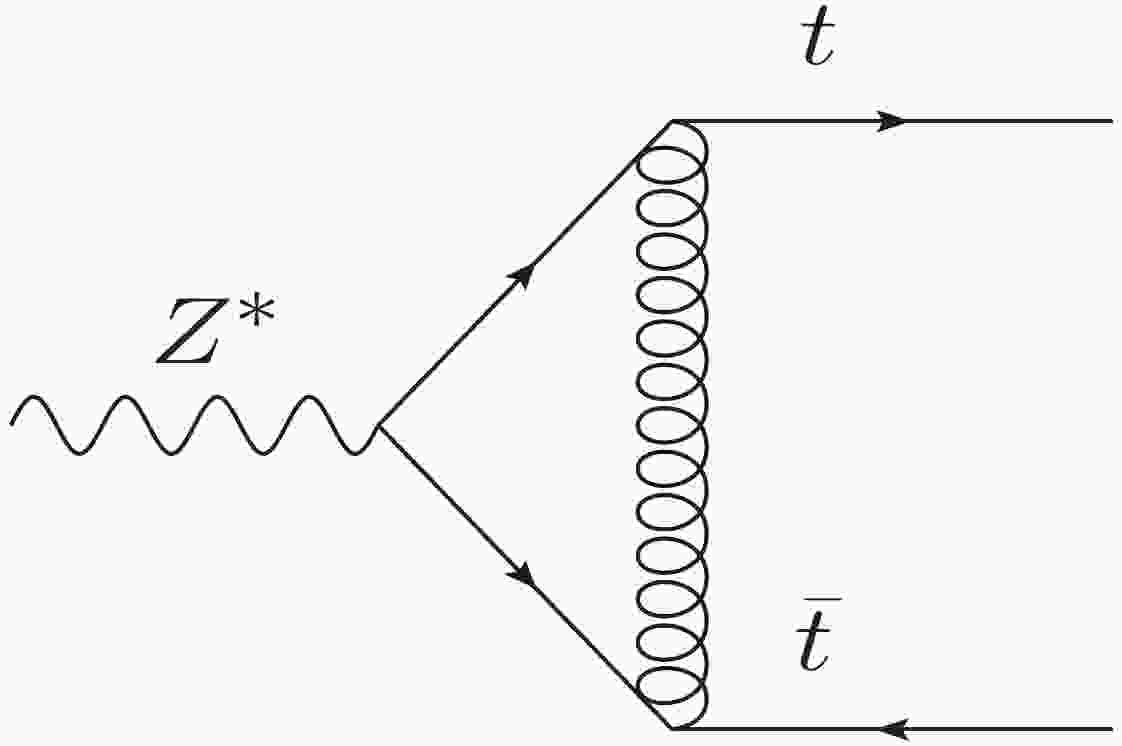
In this section, we take the one-loop amplitude reduction to demonstrate our method. We consider the one-loop diagram for
$ Z^* (k_1)\rightarrow t(k_2)\bar{t}(k_3) $ shown in Fig. 1. We define$ Q^2 \equiv k_1^2 $ and$ m_t $ as the mass of the top quark. The diagram is plotted using Jaxodraw [60] based on Axodraw [61].
Figure 1. One-loop triangle diagram for a virtual Z boson decaying into a top-quark pair.
The relevant amplitude can be written as
$ {\cal A} = \int {\rm d}^D q \dfrac{N(q,k_1,k_2,k_3)}{ {\cal D}_1 {\cal D}_2 {\cal D}_3 }, $

(21) where
$ q $ is the loop momentum.$ N(q,k_1,k_2,k_3) $ is the numerator of the amplitude, and the denominators are$ \begin{split} {\cal D}_1 & = q^2 -m_t^2,\\ {\cal D}_2 & = (q-k_1)^2 -m_t^2,\\ {\cal D}_3 & = (q-k_3)^2. \end{split} $

(22) Without loss of generality, we only consider the right-handed current of
$ Z^* $ . The numerator can then be chosen as$ \begin{split} N_R(q,k_1,k_2,k_3) = & -g^2_s \, \bar{u}(k_2,m_t)\gamma^a({{\not\! k}_1}-{\not\!\! q}+m_t)\\&\times{\not\! {\varepsilon}}P_R({\not \!\!q}+m_t)\gamma^a{v}(k_3,m_t). \end{split} $

(23) Following the approach in Section 2, we choose to decompose
$ v(k_3,m_t) $ ,$ \begin{split} {v}({k_3,m_t}) & = {v}_0(k_{30})+{v}_r(k_{3r}),\\ k_3& = k_{30}+\dfrac{m^2_t}{2k_{30}\cdot k_{3r}}k_{3r}. \end{split} $

(24) Since the reference momentum
$ k_{3r} $ has been added, we define two scalar products,$ \begin{split} s_1 &\equiv k_{3r}\cdot k_{30}, \\ s_2 &\equiv k_{3r}\cdot k_{1}. \end{split} $

(25) Based on the monomials in the original amplitude, we obtain 12 primitive amplitudes,
$ \begin{split} {\cal M}_1 & = \int {\rm d}^D q \dfrac{\bar{u}(k_2,m_t){\not\! {\varepsilon}} v_{0}(k_{30})}{ {\cal D}_1 {\cal D}_2 {\cal D}_3 },\\ {\cal M}_{2} & = \int {\rm d}^D q \dfrac{\bar{u}(k_2,m_t){\not\! {\varepsilon}} v_{r}(k_{3r})}{ {\cal D}_1 {\cal D}_2 {\cal D}_3 },\\ {\cal M}_{3} & = \int {\rm d}^D q \dfrac{\bar{u}(k_2,m_t){\not\! {\varepsilon}}{\not\!\! q}v_{0}(k_{30})}{ {\cal D}_1 {\cal D}_2 {\cal D}_3 },\\ {\cal M}_{4} & = \int {\rm d}^D q \dfrac{\bar{u}(k_2,m_t){\not\! {\varepsilon}}{\not\!\! q}v_{r}(k_{3r})}{ {\cal D}_1 {\cal D}_2 {\cal D}_3 },\\ {\cal M}_{5}& = \int {\rm d}^D q \dfrac{(k_3\cdot\varepsilon)\bar{u}(k_2,m_t)v_{0}(k_{30})}{ {\cal D}_1 {\cal D}_2 {\cal D}_3 },\\ {\cal M}_{6}& = \int {\rm d}^D q \dfrac{(k_3\cdot\varepsilon)\bar{u}(k_2,m_t)v_{r}(k_{3r})}{ {\cal D}_1 {\cal D}_2 {\cal D}_3 },\\ {\cal M}_{7}& = \int {\rm d}^D q \dfrac{(k_3\cdot\varepsilon)\bar{u}(k_2,m_t){\not\!\! q}v_{0}(k_{30})}{ {\cal D}_1 {\cal D}_2 {\cal D}_3 },\\ {\cal M}_{8}& = \int {\rm d}^D q \dfrac{(k_3\cdot\varepsilon)\bar{u}(k_2,m_t){\not\!\! q}v_{r}(k_{3r})}{ {\cal D}_1 {\cal D}_2 {\cal D}_3 },\\ {\cal M}_{9}& = \int {\rm d}^D q \dfrac{(q\cdot\varepsilon)\bar{u}(k_2,m_t)v_{0}(k_{30})}{ {\cal D}_1 {\cal D}_2 {\cal D}_3 },\\ {\cal M}_{10}& = \int {\rm d}^D q \dfrac{(q\cdot\varepsilon)\bar{u}(k_2,m_t)v_{r}(k_{3r})}{ {\cal D}_1 {\cal D}_2 {\cal D}_3 },\\ {\cal M}_{11}& = \int {\rm d}^D q \dfrac{(q\cdot\varepsilon)\bar{u}(k_2,m_t){\not\!\! q}v_{0}(k_{30})}{ {\cal D}_1 {\cal D}_2 {\cal D}_3 },\\ {\cal M}_{12}& = \int {\rm d}^D q \dfrac{(q\cdot\varepsilon)\bar{u}(k_2,m_t){\not\!\! q}v_{r}(k_{3r})}{ {\cal D}_1 {\cal D}_2 {\cal D}_3 }. \end{split} $

(26) According to the Lorentz structure, one needs four linear independent form factors,
$ \begin{split} F_{1} & = \bar{u}(k_2,m_t){\not \!\!{\varepsilon}} v_{0}(k_{30}),\\ F_{2} & = \bar{u}(k_2,m_t){\not\!\! {\varepsilon}} v_{r}(k_{3r}),\\ F_{3} & = (k_3\cdot\varepsilon)\bar{u}(k_2,m_t)v_{0}(k_{30}),\\ F_{4} & = (k_3\cdot\varepsilon)\bar{u}(k_2,m_t)v_{r}(k_{3r}). \end{split} $

(27) The primitive amplitudes can then be projected on the form factors
$ \begin{align} {\cal M}_{p} = d_{1,p}F_{1}+d_{2,p}F_{2}+d_{3,p}F_{3}+d_{4,p}F_{4}. \end{align} $

(28) Since the spinors
$ v_{0}(k_{30}) $ and$ v_{r}(k_{3r}) $ are not fully independent, relations can be found to cancel the reference momenta in the final result. For example, we note that the only difference between$ {\cal M}_{3} $ and$ {\cal M}_{4} $ is the last spinor,$ \begin{split} {\cal M}_{3} & = \int {\rm d}^D q \dfrac{\bar{u}(k_2,m_t){\not \!\!{\varepsilon}}{\not\!\! q}v_{0}(k_{30})}{ {\cal D}_1 {\cal D}_2 {\cal D}_3 },\\ {\cal M}_{4} & = \int {\rm d}^D q \dfrac{\bar{u}(k_2,m_t){\not \!\!{\varepsilon}}{\not\!\! q}v_{r}(k_{3r})}{ {\cal D}_1 {\cal D}_2 {\cal D}_3 }. \end{split} $

(29) By observing the symmetry between
$ v_{0}(k_{30}) $ and$ v_{r}(k_{3r}) $ $ \begin{split} {{\not\! k}_3}v_{0}(k_{30}) = -m_t v_{r}(k_{3r}),\quad {{\not\! k}_3}v_{r}(k_{3r}) = -m_t v_{0}(k_{30}), \end{split} $

(30) we find the relations
$ d_{3,1} = d_{4,2},\quad d_{3,2} = d_{4,1},\quad d_{3,3} = d_{4,4},\quad d_{3,4} = d_{4,3}. $

(31) Using these relations, we obtain
$ \begin{split} {k_{3r}} \cdot {{q}} = &\dfrac{2}{Q^4-4 {m^2_t} {Q^2}}\Big \{({k_2}\cdot {{q}} ) ({Q^2} {s_1}-2 {m^2_t} {s_2})\\ &+({k_3}\cdot {{q}} )({Q^2} ({s_2}-{s_1})-2 {m^2_t} {s_2})\Big\}. \end{split} $

(32) After projection of the primitive amplitudes, we also need to decompose
$ k_2 $ in each form factor as$ \begin{split} {u}({k_2,m_t}) & = {u}_0(k_{20})+{u}_r(k_{2r}),\\ k_2& = k_{20}+\dfrac{m^2_t}{2k_{20}\cdot k_{2r}}k_{2r}. \end{split} $

(33) The explicit expressions for
$ {\mathbb P}_H F_i $ can then be written in spinor representation as$ \begin{split} {\mathbb P}_{-+} F_1 & = \left\langle k_{20}|{\not\!\! {\varepsilon}}|k_{30}\right],\\ {\mathbb P}_{++} F_1 & = \dfrac{m_t}{\left\langle k_{2r}|k_{20}\right\rangle}\left\langle k_{2r}|{\not\!\! {\varepsilon}}|k_{30}\right],\\ {\mathbb P}_{++} F_2 & = -\dfrac{m_t}{\left\langle k_{30}|k_{3r}\right\rangle} \left[k_{20}|{\not\!\! {\varepsilon}}|k_{3r}\right\rangle,\\ {\mathbb P}_{-+} F_2 & = -\dfrac{m_t^2}{\left[k_{2r}|k_{20}\right]\left\langle k_{30}|k_{3r}\right\rangle} \left[k_{2r}|{\not\!\! {\varepsilon}}|k_{3r}\right\rangle,\\ {\mathbb P}_{++} F_3 & = (k_3\cdot\varepsilon)\left[k_{20}|k_{30}\right],\\ {\mathbb P}_{-+} F_3 & = (k_3\cdot\varepsilon)\dfrac{m_t}{\left[k_{2r}|k_{20}\right]}\left[k_{2r}|k_{30}\right],\\ {\mathbb P}_{-+} F_4 & = -(k_3\cdot\varepsilon) \dfrac{m_t}{\left\langle k_{30}|k_{3r}\right\rangle} \left\langle k_{20}|k_{3r}\right\rangle,\\ {\mathbb P}_{++} F_4 & = -(k_3\cdot\varepsilon) \dfrac{m_t^2}{\left\langle k_{2r}|k_{20}\right\rangle\left\langle k_{30}|k_{3r}\right\rangle}\left\langle k_{2r}|k_{3r}\right\rangle,\\ {\mathbb P}_{+-} F_1 & = \left[k_{20}|{\not \!\!{\varepsilon}}| k_{30} \right\rangle ,\\ {\mathbb P}_{--} F_1 & = \dfrac{m_t}{\left[ k_{2r}|k_{20}\right]} \left[k_{2r}|{\not\!\! {\varepsilon}} |k_{30}\right\rangle,\\ {\mathbb P}_{--} F_2 & = -\dfrac{m_t}{\left[ k_{30}|k_{3r}\right]} \left\langle k_{20}|{\not\!\! {\varepsilon}}|k_{3r}\right],\\ {\mathbb P}_{+-} F_2 & = -\dfrac{m_t^2}{\left\langle k_{2r}|k_{20}\right\rangle \left[ k_{30}|k_{3r}\right]} \left\langle k_{2r}|{\not \!\!{\varepsilon}}| k_{3r}\right],\\ {\mathbb P}_{--} F_3 & = (k_3\cdot\varepsilon)\left\langle k_{20}|k_{30} \right\rangle,\\ {\mathbb P}_{+-} F_3 & = (k_3\cdot\varepsilon)\dfrac{m_t}{\left\langle k_{2r}|k_{20}\right\rangle} \left\langle k_{2r}|k_{30} \right\rangle,\\ {\mathbb P}_{+-} F_4 & = -(k_3\cdot\varepsilon) \dfrac{m_t}{\left[ k_{30}|k_{3r}\right]} \left[ k_{20}|k_{3r}\right],\\ {\mathbb P}_{--} F_4 & = -(k_3\cdot\varepsilon) \dfrac{m_t^2}{\left[ k_{2r}|k_{20}\right]\left[ k_{30}|k_{3r}\right]} \left[ k_{2r}|k_{3r}\right]. \end{split} $

(34) The coefficients
$ c_{i,H} $ are$ \begin{align} c_{1,-+} = &c_{1,++} = c_{2,--} = c_{2,+-} \\ = &\dfrac{-g^2_s}{Q^4-4 m^2_{t} Q^2} \int {\rm d}^D q \dfrac{1}{ {\cal D}_1 {\cal D}_2 {\cal D}_3 }\big\{8 m^4_{t} Q^2-2 m^2_{t} Q^4+\left(8 (D-4) m^4_{t}-4 m^2_{t} Q^2\right) (k_2 \cdot q )+(8 (D-4) m^4_{t}-4 (D-5) m^2_{t} Q^2)(k_3 \cdot q )\big\},\\ \\ c_{2,++} = &c_{2,-+} = c_{1,+-} = c_{1,--} \\ = & \dfrac{-g^2_s}{Q^4-4 m^2_{t} Q^2} \int {\rm d}^D q \dfrac{1}{ {\cal D}_1 {\cal D}_2 {\cal D}_3 }\big\{(D-4) m^2_{t} Q^2 \left(Q^2-4 m^2_{t}\right)+(8 (D-4) m^4_{t}-4 (D-1)m^2_{t} Q^2+4 Q^4)(k_2 \cdot q )\\&+\left(8 (D-4) m^4_{t}+4 (7-2 D) m^2_{t} Q^2+2 (D-4) Q^4\right) (k_3 \cdot q )+\left(16 m^2_{t}-8 Q^2\right)(k_2 \cdot q ) (k_3 \cdot q )\\&+8 m^2_{t} (k_2 \cdot q )^2+8 m^2_{t} (k_3 \cdot q )^2 -(D-4) Q^2\left(Q^2-4 m^2_{t}\right) q^2\big\},\\ \\ c_{3,++} = & c_{3,-+} = c_{4,+-} = c_{4,--} \\ = & \dfrac{-g^2_s}{\left(Q^3-4 m^2_t Q\right)^2}\int {\rm d}^D q \dfrac{1}{ {\cal D}_1 {\cal D}_2 {\cal D}_3 }\big\{2(D-4) m_{t} \left(Q^3-4 m^2_{t} Q\right)^2+(-32 (D-4) m_{t}^5+8 \,D\, m^3_{t} Q^2-8 m_{t} Q^4)(k_2 \cdot q )\\&-4 m_{t} \left(4 m^2_{t}-Q^2\right) \left(2 (D-4) m^2_{t}-(D-6) Q^2\right) (k_3 \cdot q )+\left(8\, D \,m_{t} Q^2-32 m^3_{t}\right)(k_2 \cdot q ) (k_3 \cdot q )\\&+\left(16 (D-3) m^3_{t}-8 (D-2) m_{t} Q^2\right) (k_2 \cdot q )^2-16 (D-1) m^3_{t} (k_3 \cdot q)^2-4 m_{t} Q^2\left(Q^2-4 m^2_{t}\right) q^2\big\},\\ \\ c_{4,-+} = & c_{4,++} = c_{3,--} = c_{3,+-} \\ = & \dfrac{-g^2_s}{\left(Q^3-4 m^2_t Q\right)^2}\int {\rm d}^D q \dfrac{1}{ {\cal D}_1 {\cal D}_2 {\cal D}_3 }\big\{-8 (D-4) m^3_{t} \left(4 m^2_{t}-Q^2\right) (k_2 \cdot q )-4 (D-4) m_{t} (8 m^4_{t}-6 m^2_{t} Q^2 +Q^4) (k_3 \cdot q )\\&+\left(8\,D\,m_{t} Q^2-32 m^3_{t}\right) (k_2 \cdot q ) (k_3 \cdot q )-16 (D-1) m^3_{t}(k_2 \cdot q )^2 +\left(16 (D-3) m^3_{t}-8 (D-2) m_{t} Q^2\right) (k_3 \cdot q )^2\\&-4 m_{t} Q^2 \left(Q^2 -4 m^2_{t}\right)q^2\big\}. \end{align} $

(35) The above result was cross-checked by Tarasov’s method [41] using FaRe [62] and LiteRed [29].
-
In this Section, we take a two-loop diagram to demonstrate how our method can be used for higher order corrections. A typical two-loop diagram for
$ Z^*(k_1)\rightarrow t(k_2)\bar{t}(k_3) $ is shown in Fig. 2. Its relevant amplitude can be written as
Figure 2. Two-loop triangle diagram for a virtual Z boson decaying into a top-quark pair.
$ {\cal A} = \int {\rm d}^D q_1 {\rm d}^D q_2 \dfrac{N(q_1,q_2,k_1,k_2,k_3)}{ {\cal D}_1 {\cal D}_2 {\cal D}_3 {\cal D}_4 {\cal D}_5 {\cal D}_6 }, $

(36) where
$ q_1 $ and$ q_2 $ are the loop momenta.$ N(q_1,q_2,k_1,k_2,k_3) $ is the numerator of the two-loop amplitude. The loop denominators are$ \begin{split} {\cal D}_1 & = (q_2+k_2)^2 -m_t^2,\\ {\cal D}_2 & = (q_1)^2 - m_t^2,\\ {\cal D}_3 & = (q_1-k_1)^2 ,\\ {\cal D}_4 & = (q_2-k_3)^2 - m_t^2,\\ {\cal D}_5 & = (q_2)^2,\\ {\cal D}_6 & = (q_1-q_2-k_2)^2. \end{split} $

(37) To complete the integral family for the above two-loop amplitude, an additional denominator is needed
$ {\cal D}_7 = (q_1-k_2)^2. $

(38) Without loss of generality, we only consider the right-handed current of
$ Z^* $ . The numerator can then be chosen as$ \begin{split} N_R(&q_1,q_2,k_1,k_2,k_3) = g^4_s \bar{u}(k_2)\gamma^a({{\not\!\! q}_2}+{{\not\!\! k}_2}+m_t)\gamma^b({{\not\!\! q}_1}+m_t)\\ &\times {\not\!\! {\varepsilon}}P_R({{\not \!\!k}_1}-{{\not\!\! q}_1}+m_t) \gamma^b ({{\not\!\! k}_3}-{{\not \!\!q}_2}+m_t)\gamma^a v(k_3). \end{split} $

(39) We choose to decompose
$ v(k_3,m_t) $ and define two additional scalar products,$ \begin{split} s_1 \equiv k_{3r}\cdot k_{30},\quad s_2 \equiv k_{3r}\cdot k_{1} . \end{split} $

(40) We then obtain four linear independent form factors
$ \begin{split} F_{1} & = \bar{u}(k_2,m_t){\not\!\! {\varepsilon}} v_{0}(k_{30}),\quad F_{2} = \bar{u}(k_2,m_t){\not\!\! {\varepsilon}} v_{r}(k_{3r}),\\ F_{3} & = (k_3\cdot\varepsilon)\bar{u}(k_2,m_t)v_{0}(k_{30}),\\ F_{4} & = (k_3\cdot\varepsilon)\bar{u}(k_2,m_t)v_{r}(k_{3r}). \end{split} $

(41) Similarly to the one-loop case, we find the relations,
$ \begin{split} {k_{3r}} \cdot {{q_1}} = & \dfrac{2}{Q^4-4 {m^2_t} Q^2} \{({k_2}\cdot {{q_1}} ) ({Q^2} {s_1}-2 {m^2_t} {s_2})\\ &+({k_3}\cdot {{q_1}} )({Q^2} ({s_2}-{s_1})-2 {m^2_t} {s_2})\}, \end{split} $

(42) $ \begin{split} \\ {k_{3r}} \cdot {{q_2}} = & \dfrac{2}{Q^4-4 {m^2_t} Q^2} \{({k_2}\cdot {{q_2}} ) ({Q^2} {s_1}-2 {m^2_t} {s_2})\\ &+({k_3}\cdot {{q_2}} )({Q^2} ({s_2}-{s_1})-2 {m^2_t} {s_2})\}. \end{split} $

(43) After projection of the primitive amplitudes, one needs to decompose
$ k_2 $ in each form factor. The explicit expressions for$ {\mathbb P}_H F_i $ can be written in spinor representation as$ \begin{split} {\mathbb P}_{-+} F_1 & = \left\langle k_{20}|{\not \!\! {\varepsilon}}|k_{30}\right],\\ {\mathbb P}_{++} F_1 & = \dfrac{m_t}{\left\langle k_{2r}|k_{20}\right\rangle}\left\langle k_{2r}|{\not \!\! {\varepsilon}}|k_{30}\right],\\ {\mathbb P}_{++} F_2 & = -\dfrac{m_t}{\left\langle k_{30}|k_{3r}\right\rangle} \left[k_{20}|{\not \!\! {\varepsilon}}|k_{3r}\right\rangle,\\ {\mathbb P}_{-+} F_2 & = -\dfrac{m_t^2}{\left[k_{2r}|k_{20}\right]\left\langle k_{30}|k_{3r}\right\rangle} \left[k_{2r}|{\not \!\! {\varepsilon}}|k_{3r}\right\rangle,\\ {\mathbb P}_{++} F_3 & = (k_3\cdot\varepsilon)\left[k_{20}|k_{30}\right],\\ {\mathbb P}_{-+} F_3 & = (k_3\cdot\varepsilon)\dfrac{m_t}{\left[k_{2r}|k_{20}\right]}\left[k_{2r}|k_{30}\right], \end{split} $

$ \begin{split} {\mathbb P}_{-+} F_4 & = -(k_3\cdot\varepsilon) \dfrac{m_t}{\left\langle k_{30}|k_{3r}\right\rangle} \left\langle k_{20}|k_{3r}\right\rangle,\\ {\mathbb P}_{++} F_4 & = -(k_3\cdot\varepsilon) \dfrac{m_t^2}{\left\langle k_{2r}|k_{20}\right\rangle\left\langle k_{30}|k_{3r}\right\rangle}\left\langle k_{2r}|k_{3r}\right\rangle,\\ {\mathbb P}_{+-} F_1 & = \left[k_{20}|{\not \!\! {\varepsilon}}| k_{30} \right\rangle ,\\ {\mathbb P}_{--} F_1 & = \dfrac{m_t}{\left[ k_{2r}|k_{20}\right]} \left[k_{2r}|{\not \!\! {\varepsilon}} |k_{30}\right\rangle,\\ {\mathbb P}_{--} F_2 & = -\dfrac{m_t}{\left[ k_{30}|k_{3r}\right]} \left\langle k_{20}|{\not \!\! {\varepsilon}}|k_{3r}\right],\\ {\mathbb P}_{+-} F_2 & = -\dfrac{m_t^2}{\left\langle k_{2r}|k_{20}\right\rangle \left[ k_{30}|k_{3r}\right]} \left\langle k_{2r}|{\not \!\! {\varepsilon}}| k_{3r}\right],\\ {\mathbb P}_{--} F_3 & = (k_3\cdot\varepsilon)\left\langle k_{20}|k_{30} \right\rangle,\\ {\mathbb P}_{+-} F_3 & = (k_3\cdot\varepsilon)\dfrac{m_t}{\left\langle k_{2r}|k_{20}\right\rangle} \left\langle k_{2r}|k_{30} \right\rangle,\\ {\mathbb P}_{+-} F_4 & = -(k_3\cdot\varepsilon) \dfrac{m_t}{\left[ k_{30}|k_{3r}\right]} \left[ k_{20}|k_{3r}\right],\\ {\mathbb P}_{--} F_4 & = -(k_3\cdot\varepsilon) \dfrac{m_t^2}{\left[ k_{2r}|k_{20}\right]\left[ k_{30}|k_{3r}\right]} \left[ k_{2r}|k_{3r}\right]. \end{split} $

(44) In order to simplify the coefficients
$ c_{i,H} $ , we use$ x_i $ to denote seven linear independent scalar products$ \begin{split} x_1 & = q_1 \cdot k_2,\quad x_2 = q_1 \cdot k_3,\\ x_3 & = q_2 \cdot k_2,\quad x_4 = q_2 \cdot k_3,\\ x_5 & = q_1^2,\quad x_6 = q_2^2,\quad x_7 = q_1 \cdot q_2. \end{split} $

(45) $ \begin{split} c_{1,-+} = &c_{1,++} = c_{2,--} = c_{2,+-} = \dfrac{2g^4_s {m^2_t}}{(D-2) {Q^2} \left(Q^2-4 {m^2_t}\right)}\int {\rm d}^D q_1 {\rm d}^D q_2 \dfrac{1}{ {\cal D}_1 {\cal D}_2 {\cal D}_3 {\cal D}_4 {\cal D}_5 {\cal D}_6 }\\& \times \Big\{ -16 (D-2) m^2_{t} x_1^2 +8 (D-2) x_4 x_1^2 -16 (D-2) m^2_{t} x_2^2 -4 \left(D^3-16 D^2+80 D-124\right) x_1 x_4^2 \\& +4 \left(D^3-12 D^2+44 D-52\right) m^2_{t} x_4^2 -4 (D-3) (D-2) Q^2 \left(Q^2-4 m^2_{t}\right) x_1 -4 (D-2) Q^2 \left(Q^2-4 m^2_{t}\right) x_2 \\& -2 Q^2 \left(2 D^2-19 D+38\right) \left(Q^2-4 m^2_{t}\right) x_7 +2 (D-4)(D-2) \left(Q^2-4 m^2_{t}\right) Q^2 x_5\\& +(D-4) \left(D^2-6 D+10\right) \left(Q^2-4 m^2_{t}\right) Q^2 x_6 +4 (D-4) \left((D-4)^2 m^2_{t}-(D-5) Q^2\right) x_1 x_6 \\& +2 (D-4) \left(2 (D-4)^2 m^2_{t}-\left(D^2-10 D+26\right) Q^2\right) x_2 x_6 +2 (D-2) \left(Q^2-4 m^2_{t}\right) Q^2 \left((D-2) m^2_{t}-Q^2\right) \\& + \left(4 \left(D^3-12 D^2+44 D-52\right) m^2_{t} -2 (D-4)^2 (D-2) Q^2\right)x_3^2 +4 \left(D^3-14 D^2+64 D-92\right) x_2 x_3^2 \\& +16 (D-2) \left(Q^2-2 m^2_{t}\right) x_1 x_2 -8 (D-2) x_1 x_2 x_3 +8 (D-5) (D-2) x_2^2 x_3 +2 (D-4) (D-2) \left(2 (D-4) m^2_{t}-Q^2\right) x_3 x_5 \\& +2 (D-2) \left(2 (D-4) (D-2) m^4_{t}+\left(-4 D^2+25 D-42\right) Q^2 m^2_{t}+\left(D^2-7 D+14\right) Q^4\right) x_3 \\& +\left(4 (D-4) (D-2) Q^2-8 \left(2 D^2-19 D+38\right) m^2_{t}\right) x_1 x_3 \\& +\left(8 \left(D^3-12 D^2+51 D-70\right) m^2_{t} -4 \left(D^3-11 D^2+43 D-58\right) Q^2\right) x_2 x_3 \\& +2 (D\!-\!4) (D\!-\!2) \left(2 (D\!-\!4) m^2_{t}-(D\!-\!5) Q^2\right) x_4 x_5 +2 (D-2) \left(2 (D-4) (D-2) m^4_{t}-\left(D^2-9 D+14\right) Q^2 m^2_{t}-2 Q^4\right) x_4 \\& +\left(4 \left(D^3-10 D^2+25 D-10\right) Q^2-8 (D-3) \left(D^2-5 D-2\right) m^2_{t}\right) x_1 x_4 \\& +\left(8 (D-5) (D-2) Q^2 -8 \left(2 D^2-19 D+38\right) m^2_{t}\right) x_2 x_4 -8 (D-5) (D-2) x_1 x_2 x_4 \\& +\left(8 \left(D^3-12 D^2+44 D-52\right) m^2_{t} -2 \left(D^3-14 D^2+56 D-72\right) Q^2\right) x_3 x_4 -4 \left(D^3-14 D^2+64 D-92\right) x_1 x_3 x_4 \\& +4 \left(D^3\!-\!16 D^2\!+\!80 D\!-\!124\right) x_2 x_3 x_4 \!+\!4 (D\!-\!2) \left(2 (D-4) m^2_{t}\!-\!Q^2\right) x_1 x_7 +4 (D-2) \left(2 (D-4) m^2_{t}-(D-5) Q^2\right) x_2 x_7 \\& -8 (D-3) \left((D-4)^2 m^2_{t}-(D-5) Q^2\right) x_3 x_7-4 (D-3) \left(2 (D-4)^2 m^2_{t}-\left(D^2-10 D+26\right) Q^2\right) x_4 x_7 \Big\}, \end{split} $

(46) $ \begin{split} c_{2,++} = &c_{2,-+} = c_{1,+-} = c_{1,--} = \dfrac{g^4_s}{(D-2)Q^2(Q^2-4m^2_t)}\int {\rm d}^D q_1 {\rm d}^D q_2 \dfrac{1}{ {\cal D}_1 {\cal D}_2 {\cal D}_3 {\cal D}_4 {\cal D}_5 {\cal D}_6 }\\ &\times\Big\{ 8 (D-4)^2 (D-3) m^4_{t} x_3^2 +4 (D-2) \left(2 (D-4) (D-2) m^2_{t}+(14-3 D) Q^2\right) m^4_{t} x_4 -16 (D-2)\left(2 m^2_{t}-Q^2\right) m^2_{t}x_2^2 \\& -8 (D-2)^2 m^2_{t} x_3^2 x_5 -8 (D-2)^2 m^2_{t} x_4^2 x_5 -8 (D-2)^2 m^2_{t} x_1^2 x_6 -8 (D-2)^2 m^2_{t} x_2^2 x_6 -(D-4)^3 Q^2 m^2_{t} \left(4 m^2_{t}-Q^2\right) x_6 \\& +16 (D-2) \left(Q^2-2 m^2_{t}\right) m^2_{t}x_1^2 -2 (D-2) Q^2 m^2_{t} \left(4 m^2_{t}-Q^2\right) \left(2 (D-2) m^2_{t}-(D-4) Q^2\right)\\& +4 (D-4)^2 \left(2 (D-3) m^2_{t}-(D-2) Q^2\right) m^2_{t}x_4^2\\& +4 (D-2) \left(2 (D-4) (D-2) m^4_{t}-(D-3) (D-2) Q^2 m^2_{t}+(D-4) Q^4\right)m^2_{t} x_3 \\& +4 (D-4)^2 m^2_{t} \left(4 (D-3) m^2_{t}-(D-4) Q^2\right) x_3 x_4 +16 (D-2)^2 m^2_{t} x_1 x_3 x_7 +16 (D-2)^2 m^2_{t} x_2 x_4 x_7 \\& -16 (D-2) \left(3 m^2_{t}-Q^2\right) x_3 x_2^2 +4 (D-2)^2 \left(Q^2-4 m^2_{t}\right) Q^2 x_7^2 -2 (D-4) (D-2) Q^2 \left(8 m^4_{t}-6 Q^2 m^2_{t}+Q^4\right) x_5\\& -8 (D-2)^2 \left(2 m^2_{t}-Q^2\right) x_3 x_4 x_5 +(D-6) (D-2)^2 \left(Q^2-4 m^2_{t}\right) Q^2 x_5 x_6\\& +2 (D-4)\left(4 (D-4)^2 m^4_{t} +2 \left(D^2-6 D+14\right) Q^2 m^2_{t}-\left(D^2-8 D+20\right) Q^4\right) x_1 x_6\\& +8 (D-4) \left((D-4)^2 m^4_{t} +(3 D-11) Q^2 m^2_{t}-(D-4) Q^4\right) x_2 x_6 -8 (D-2)^2 \left(2 m^2_{t}-Q^2\right) x_1 x_2 x_6 \\& +\left(4 \left(D^3-14 D^2+68 D-104\right) Q^2-8 \left(D^3-16 D^2+80 D-124\right) m^2_{t}\right) x_1 x_4^2 \\& +4 (D-2) Q^2 \left(4 m^2_{t}-Q^2\right) \left(2 (D-3) m^2_{t}-(D-4) Q^2\right) x_1\\& + \left(8 \left(D^3-14 D^2+64 D-92\right) m^2_{t}-4 (D-4) \left(D^2-12 D+28\right) Q^2\right) x_2 x_3^2 +8 (D-2) Q^2 \left(4 m^4_{t}-5 Q^2 m^2_{t}+Q^4\right) x_2 \\& -16 (D-2) \left(Q^2-2 m^2_{t}\right)^2 x_1 x_2 -16 (D-2) \left((D-1) m^2_{t}-Q^2\right) x_1 x_2 x_3 \\& +4 (D-4) (D-2) \left(2 (D-4) m^4_{t} -(D-1) Q^2 m^2_{t}+Q^4\right) x_3 x_5 \\& +\left(-16 \left(3 D^2-21 D+38\right) m^4_{t}+16 (3 D-8) (D-4) Q^2 m^2_{t} -8 (D-4) (D-2) Q^4\right) x_1 x_3 \\& +\left(16 \left(D^3-13 D^2+53 D-70\right) m^4_{t}+8 \left(5 D^2-35 D+66\right) Q^2 m^2_{t} -8 \left(D^2-7 D+14\right) Q^4\right) x_2 x_3 \\& -16 (D-2) \left(Q^2-(D-1) m^2_{t}\right) x_1^2 x_4 +4 (D-4) (D-2) \left(2 (D-4) m^4_{t}+3 Q^2 m^2_{t}-Q^4\right) x_4 x_5 \\& -8 \left(2 \left(D^3-7 D^2+11 D+6\right) m^4_{t}+\left(-2 D^2+23 D-54\right) Q^2 m^2_{t}+(10-3 D) Q^4\right) x_1 x_4 \\& +\left(-16 \left(3 D^2-21 D+38\right) m^4_{t}+8 \left(D^2-16 D+36\right) Q^2 m^2_{t} +16 (D-2) Q^4\right) x_2 x_4 +16 (D-2) \left(3 m^2_{t}-Q^2\right) x_1 x_2 x_4 \\& +\left(4 (D-4) \left(D^2-12 D+28\right) Q^2 -8 \left(D^3-14 D^2+64 D-92\right) m^2_{t}\right) x_1 x_3 x_4 \\& +\left(8 \left(D^3-16 D^2+80 D-124\right) m^2_{t} -4 \left(D^3-14 D^2+68 D-104\right) Q^2\right) x_2 x_3 x_4 \\& +4 \left((D-6) (D-3) Q^6+(7 D-22) (5-D) m^2_{t} Q^4 +4 \left(3 D^2-21 D+38\right) m^4_{t} Q^2\right) x_7 \\& +8 (D-2) \left(2 (D-4) m^4_{t}-(D-1) Q^2 m^2_{t}+Q^4\right) x_1 x_7 +8 (D-2) \left(2 (D-4) m^4_{t}+3 Q^2 m^2_{t}-Q^4\right) x_2 x_7 \\& +2 \left(-8 (D-4)^2 (D-3) m^4_{t} +4 \left(3 D^2-20 D+34\right) Q^2 m^2_{t}+(D-4) \left(D^2-12 D+28\right) Q^4\right) x_3 x_7 \\& +8 (D-2)^2 \left(2 m^2_{t}-Q^2\right)x_2 x_3 x_7 +8 (D-2)^2 \left(2 m^2_{t}-Q^2\right) x_1 x_4 x_7 \\& -2 \left(8 (D-4)^2 (D-3) m^4_{t}-4 \left(D^3-12 D^2+52 D-74\right) Q^2 m^2_{t} +\left(D^3-14 D^2+68 D-104\right) Q^4\right) x_4 x_7 \Big\}, \end{split} $

(47) $ \begin{split} c_{3,++} = & c_{3,-+} = c_{4,+-} = c_{4,--} = \dfrac{4m_t g^4_s}{(D-2)(Q^3-4m^2_tQ)^2}\int {\rm d}^D q_1 {\rm d}^D q_2 \dfrac{1}{ {\cal D}_1 {\cal D}_2 {\cal D}_3 {\cal D}_4 {\cal D}_5 {\cal D}_6 }\\ &\times\Big\{ -2 (D-2)^2 \left(Q^2-4 m^2_t\right) Q^2 x_7^2 +4 (D-1)(D-2)^2 m^2_t x_5 x_4^2 +2 (D-2)^2 \left((D-2) Q^2-2 (D-3) m^2_t\right) x_5 x_3^2 \\& -2 (D-2)^2 \left(D Q^2-4 m^2_t\right) x_3 x_4 x_5 +4 (D-1) (D-2)^2 m^2_t x_6 x_2^2 +2 (D-2)^2 \left(Q^2-4 m^2_t\right) Q^2 x_5 x_6 \\& +2 (D-2)^2 \left((D-2) Q^2-2 (D-3) m^2_t\right) x_6 x_1^2 -2 (D-2)^2 \left(D Q^2-4 m^2_t\right) x_1 x_2 x_6 -4 (D-1)(D-2)^2 \left(2 m^2_t-Q^2\right) x_2 x_3 x_7 \\ & +4 (D-2)^2 \left(2 (D-3) m^2_t-(D-2) Q^2\right) x_1 x_3 x_7 +4 (D-2)^2 \left(2 (D-3) m^2_t+Q^2\right) x_1 x_4 x_7 -8 (D-1)(D-2)^2 m^2_t x_2 x_4 x_7 \end{split} $

$ \begin{split} & +2 (D-3)(D-2) \left(Q^3-4 m^2_t Q\right)^2 x_5 -2 (D-2) \left(4 m^2_t-Q^2\right) \left(2 \left(D^2-6 D+10\right) m^2_t-(D-3) D Q^2\right) x_3 x_5\\ & -4 (D-2)\left(4 m^2_t-Q^2\right) \left(\left(D^2-6 D+10\right) m^2_t+(D-3) Q^2\right) x_4 x_5 +8 (D-2) m^2_t \left(4 m^2_t-Q^2\right) x_2^2 \\& +4 (D-2) \left(4 m^2_t-Q^2\right) \left(2 m^2_t-(D-2) Q^2\right) x_1^2 -2 (D-4)(D-2) Q^2 \left(8 m^4_t-6 Q^2 m^2_t+Q^4\right) x_1 \\& +4 (D-2) \left(Q^2-4 m^2_t\right) Q^2 \left((D+4) m^2_t-2 Q^2\right) x_2 +4 (D-2)\left(4 m^2_t-Q^2\right) \left(4 m^2_t+(D-4) Q^2\right) x_1 x_2 \\& -4 (D-4)(D-2)(D-1) \left(2 m^2_t-Q^2\right) x_1 x_2 x_3 +2 (D-2) m^2_t \left(4 m^2_t-Q^2\right) \left(2 (D-2) m^2_t+(D-4)^2 Q^2\right) x_3 \\& +4 (D-2) \left(2 \left(D^2-5 D+12\right) m^2_t -\left(D^2-5 D+8\right) Q^2\right) x_3 x_2^2 +4 (D-4) (D-2) (D-1) \left(2 m^2_t-Q^2\right) x_4 x_1^2\\& +2 (D-2) m^2_t \left(8 (D-2) m^4_t-2 \left(2 D^2-13 D+26\right) Q^2 m^2_t+\left(D^2-7 D+14\right) Q^4\right) x_4 \\& -4 (D-2) \left(2 \left(D^2-5 D+12\right) m^2_t-\left(D^2-5 D+8\right) Q^2\right) x_1 x_2 x_4 -2 (D-2)\left(4 m^2_t-Q^2\right) \left(2 (D-4) m^2_t +(D-3) D Q^2\right) x_1 x_7 \\& -2 (D-2)\left(8 (D-4) m^4_t+2 \left(-2 D^2+5 D+4\right) Q^2 m^2_t+(D-3) D Q^4\right) x_2 x_7 \\& -4 \left(4 \left(5 D^2-34 D+58\right) m^2_t+\left(D^3-12 D^2+50 D-68\right) Q^2\right) x_1 x_4^2 -\left(3 D^2-20 D+36\right) \left(4 m^2_t-Q^2\right) m^2_t Q^2x_6\\& +\left(-8 (D-4)^3 m^4_t+6 \left(D^3-4 D^2+16\right) Q^2 m^2_t-\left(D^3-24 D+56\right) Q^4\right) x_1 x_6\\& +\left(-8 (D-4)^3 m^4_t+2 \left(D^3-28 D^2+144 D-224\right) Q^2 m^2_t+8 \left(D^2-6 D+10\right) Q^4\right) x_2 x_6 \\& + \left(4 \left(D^3-3 D^2-8 D+28\right) m^4_t+2 (D-4)^2 (D-2) Q^2 m^2_t\right) x_3^2 \\& + \left(4 (D-2) \left(D^2-6 D+10\right) m^2_t Q^2-4 \left(D^3-9 D^2+32 D-44\right) m^4_t\right) x_4^2 \\& + \left(32 (D-3) (2 D-7) m^2_t -4 \left(D^3-3 D^2-10 D+32\right) Q^2\right) x_2x_3^2 \\& -4 \left(2 \left(D^3-15 D^2+76 D-116\right) m^4_t+(5 D-12) (D-6) Q^2 m^2_t+2 (D-2) Q^4\right) x_1 x_3 \\& +\left(-8 (D-3) \left(D^2-24 D+60\right) m^4_t-4 \left(D^3+18 D^2-114 D+172\right) Q^2 m^2_t+2 \left(D^3+D^2-22 D+40\right) Q^4\right) x_2 x_3 \\& +\left(8 \left(D^3-5 D^2-12 D+52\right) m^4_t+ 8 \left(D^3-11 D^2+47 D-70\right) Q^2 m^2_t-2 (D-4) \left(D^2-7 D+14\right) Q^4\right) x_1 x_4 \\& +\left(8 \left(D^3+7 D^2-68 D+116\right) m^4_t-4 \left(D^3+D^2-46 D+88\right) Q^2 m^2_t-16 (D-2) Q^4\right) x_2 x_4 \\& -2 \left(3 D^2-20 D+36\right) \left(D Q^2-4 m^2_t\right)m^2_t x_3 x_4 +\left(4 \left(D^3-3 D^2-10 D+32\right) Q^2 -32 (D-3) (2 D-7) m^2_t\right) x_1 x_3 x_4 \\& +4 \left(4 \left(5 D^2-34 D+58\right) m^2_t+\left(D^3-12 D^2+50 D-68\right) Q^2\right) x_2 x_3 x_4 \\& +\left((D-6) (D-4) (D-3) Q^6+2 \left(-4 D^3+51 D^2-212 D+284\right) m^2_t Q^4 +8 \left(2 D^3-25 D^2+104 D-140\right) m^4_t Q^2\right) x_7 \\& +2 (D-4) \left(4 m^2_t-Q^2\right) \left(2 (D-4) (D-3) m^2_t +(10-3 D) Q^2\right) x_3 x_7 \\& +2 \left(8 (D-4)^2 (D-3) m^4_t+2 \left(-3 D^3+35 D^2-140 D+184\right) Q^2 m^2_t +\left(D^3-12 D^2+50 D-68\right) Q^4\right) x_4 x_7 \Big\}, \end{split} $

(48) $ \begin{split} c_{4,-+} = & c_{4,++} = c_{3,--} = c_{3,+-} = \dfrac{2m_tg^4_s}{(D-2)(Q^3-4m^2_tQ)^2}\int {\rm d}^D q_1 {\rm d}^D q_2 \dfrac{1}{ {\cal D}_1 {\cal D}_2 {\cal D}_3 {\cal D}_4 {\cal D}_5 {\cal D}_6 }\\&\times \Big\{-4 (D-2)^2 \left(Q^2-4 m^2_t\right) Q^2 x_7^2 +8 (D-1) x_3^2 m^2_t x_5 (D-2)^2 +4 (D-2)^2 \left((D-2) Q^2-2 (D-3) m^2_t\right)x_4^2 x_5 \\& -4 (D-2)^2 \left(D Q^2-4 m^2_t\right) x_3 x_4 x_5 +8 (D-1) (D-2)^2 m^2_t x_6 x_1^2 +4 (D-2)^2 \left(Q^2-4 m^2_t\right) Q^2 x_5 x_6 \\& +4 (D-2)^2 \left((D-2) Q^2-2 (D-3) m^2_t\right) x_6 x_2^2-4 (D-2)^2 \left(D Q^2-4 m^2_t\right) x_1 x_2 x_6 -16 (D-1)(D-2)^2 m^2_t x_1 x_3 x_7 \\& +8 (D-2)^2 \left(2 (D-3) m^2_t+Q^2\right) x_2 x_3 x_7 -8 (D-1) (D-2)^2 \left(2 m^2_t-Q^2\right) x_1 x_4 x_7 \\& +8 (D-2)^2 \left(2 (D-3) m^2_t-(D-2) Q^2\right) x_2 x_4 x_7 -8 (D-4)(D-2) \left(2 (D+1) m^2_t-Q^2\right) x_3 x_2^2 \\& -4 (D-2)\left(Q^3-4 m^2_t Q\right)^2 x_5 +16 (D-2) m^2_t \left(4 m^2_t-Q^2\right) x_1^2 +8 (D-2)\left(4 m^2_t-Q^2\right) \left(2 m^2_t+(D-2) Q^2\right) x_2^2 \\& +2 (D-2)\left(Q^3-4 m^2_t Q\right)^2 \left(2 (D-2) m^2_t-(D-4) Q^2\right) -4 (D-2)\left(Q^2-4 m^2_t\right) \left(D \left(Q^2-2 m^2_t\right)-2 Q^2\right)Q^2 x_1 \\& +8 (D-2)\left(4 m^2_t-Q^2\right) \left((3 D-8) m^2_t-(D-3) Q^2\right)Q^2 x_2 -8 (D-2)\left(4 m^2_t-Q^2\right) \left(D Q^2-4 m^2_t\right) x_1 x_2\\ & +8 (D-2)\left(4 m^2_t-Q^2\right) \left(2 (D-3) m^2_t-Q^2\right) x_3 x_5 \end{split} $

$ \begin{split} & -4 (D-2)\left(4 m^2_t-Q^2\right) \left(2 (D-3) (D-2) m^4_t -(D-2) (D-1) Q^2 m^2_t+(D-4) Q^4\right) x_3 \\& +8 (D-2)\left(2 \left(D^2-3 D+4\right) m^2_t-D Q^2\right) x_1 x_2 x_3 +4 (D-2)\left(4 m^2_t-Q^2\right) \left(4 (D-3) m^2_t-(D-4) Q^2\right) x_4 x_5 \\& +8 (D-2) \left(D Q^2-2 \left(D^2-3 D+4\right) m^2_t\right) x_4 x_1^2 \\& -4 (D-2)\left(4 m^2_t-Q^2\right) \left(2 (D-3) (D-2) m^4_t +2 (D-2) Q^2 m^2_t-(D-4) Q^4\right) x_4 \\& +8 (D-4)(D-2) \left(2 (D+1) m^2_t-Q^2\right) x_1 x_2 x_4 -4 (D-2) \left(4 m^2_t-Q^2\right) \left(2 (D-4) m^2_t-D Q^2\right) x_1 x_7 \\& -4 (D-2)\left(4 m^2_t-Q^2\right) \left(2 (D-4) m^2_t+D Q^2\right) x_2 x_7 \\& +\left((D-4)^2 (D-2) Q^6+2 \left(-4 D^3+43 D^2-148 D+164\right) m^2_t Q^4 +8 \left(2 D^3-23 D^2+84 D-100\right) m^4_t Q^2\right) x_6 \\& +\left(-16 (D-4)^3 m^4_t-4 \left(D^3-4 D^2+24 D-64\right) Q^2 m^2_t+2 \left(D^3-8 D^2+36 D-64\right) Q^4\right) x_1 x_6 \\& -4 \left(4 (D-4)^3 m^4_t+\left(-5 D^3+44 D^2-168 D+240\right) Q^2 m^2_t+\left(D^3-8 D^2+30 D-44\right) Q^4\right) x_2 x_6 \\& + \left(16 (D-2) \left(D^2-7 D+13\right) m^2_t Q^2 -8 \left(5 D^3-49 D^2+160 D-172\right) m^4_t\right)x_3^2 \\& +\left(12 (D-4)^2 (D-2) m^2_t Q^2-8 (D-3) \left(3 D^2-28 D+52\right) m^4_t\right)x_4^2 \\& + \left(32 (D-3) \left(D^2-8 D+22\right) m^2_t-16 \left(D^3-9 D^2+31 D-38\right) Q^2\right) x_1 x_4^2 \\& -8 \left(4 \left(D^3-10 D^2+38 D-50\right) m^2_t+(3 D-10) (D-4) Q^2\right) x_2 x_3^2 \\& -4 \left(4 \left(3 D^3-23 D^2+76 D-100\right) m^4_t-4 \left(D^3-4 D^2+11 D-26\right) Q^2 m^2_t+(3 D-10) D Q^4\right) x_2 x_3 \\& +8 \left(2 \left(D^3-5 D^2-4 D+36\right) m^4_t+\left(-D^3+D^2+14 D-32\right) Q^2 m^2_t+(D-2)^2 Q^4\right) x_1 x_3 \\& +\left(16 \left(3 D^3-25 D^2+60 D-28\right) m^4_t-8 \left(D^3-12 D^2+22 D+20\right) Q^2 m^2_t-4 \left(D^2+2 D-16\right) Q^4\right) x_1 x_4 \\& -8 \left(2 (D-3) \left(D^2+12\right) m^4_t+(3 D-8) (D-6) Q^2 m^2_t-(D-4) (D-2) Q^4\right) x_2 x_4 \\& +\left(-16 \left(4 D^3-43 D^2+148 D-164\right) m^4_t+4 \left(9 D^3-100 D^2+348 D-384\right) Q^2 m^2_t-8 (D-4)^2 (D-2) Q^4\right) x_3 x_4 \\& +8 \left(4 \left(D^3-10 D^2+38 D-50\right) m^2_t+(3 D-10) (D-4) Q^2\right) x_1 x_3 x_4 \\& +\left(16 \left(D^3-9 D^2+31 D-38\right) Q^2-32 (D-3) \left(D^2-8 D+22\right) m^2_t\right) x_2 x_3 x_4 \\& -2 \left((D-6) (D-4) Q^6-2 \left(3 D^2-36 D+92\right) m^2_t Q^4+8 \left(D^2-16 D+44\right) m^4_t Q^2\right) x_7 \\& +4 (D-4) \left(4 m^2_t-Q^2\right) \left(2 (D-4) (D-3) m^2_t+(10-3 D) Q^2\right) x_3 x_7 \\& +4 \left(8 (D-4)^2 (D-3) m^4_t+2 \left(-3 D^3+35 D^2-140 D+184\right) Q^2 m^2_t+\left(D^3-12 D^2+50 D-68\right) Q^4\right) x_4 x_7\Big\}. \end{split} $

(49) To check the above results for the coefficients
$ c_{i,H} $ , we used Tarasov’s method [41] and the IBP reduction to reduce the amplitude numerically. We applied the numerical IBP reduction to the coefficients$ c_{i,H} $ and compared the two results. For the numerical check, we chose all combinations of$ (Q^2,m^2_t)\in\{(204,31),(342,76), $ $(604,131)\} $ and$ D\in\{13,17,21\} $ . After the IBP reduction by LiteRed [29], we found that all numerical expressions for the coefficients$ c_{i,H} $ are consistent with the numerical reduction results by Tarasov's method using FaRe [62] and LiteRed. For reader’s convenience, we show the explicit numerical expressions for the coefficients$ c_{i,H} $ for$ Q^2 = 204 $ ,$ m^2_t = 31 $ and$ D = 13 $ . We define$ I_{a_1,a_2,a_3,a_4,a_5,a_6,a_7} \equiv \int \dfrac{{\rm d}^D q_1 {\rm d}^D q_2}{ {\cal D}^{a_1}_1 {\cal D}^{a_2}_2 {\cal D}^{a_3}_3 {\cal D}^{a_4}_4 {\cal D}^{a_5}_5 {\cal D}^{a_6}_6 {\cal D}^{a_7}_7 }. $

(50) The numerical coefficients are
$ \begin{split} c_{1,-+} = &c_{1,++} = c_{2,--} = c_{2,+-} = \dfrac{g_s^4}{547285587552000}(-349758480361050 I_{0,0,0,1,1,1,1}+12411033570133 I_{0,0,1,1,1,0,0}\\&+561600032236650 I_{0,1,0,0,0,1,0}+54203486007512020 I_{0,1,0,1,1,1,0}-2524949213666400 I_{0,1,0,1,1,1,1}\\&-37669046330192400 I_{0,1,1,0,0,1,0}+1725030658739520 I_{0,1,1,1,1,0,0}-4392957485551487040 I_{0,1,1,1,1,1,0}\\&-43861242480409840 I_{0,2,0,1,1,1,0}-29063980357164172800 I_{0,2,1,1,1,1,0}+1620333018035519040 I_{1,1,0,1,1,1,1}\\&-72885095952847200 I_{1,1,1,1,1,0,0}+11596870539170956800 I_{2,1,0,1,1,1,1}), \end{split} $

(51) $ \begin{split} c_{2,++} = &c_{2,-+} = c_{1,+-} = c_{1,--} =\dfrac{g_s^4}{16965853214112000}(8269804372235850 I_{0,0,0,1,1,1,1}+128265951369391 I_{0,0,1,1,1,0,0}\\&-91088086096643130 I_{0,1,0,0,0,1,0}-649848399059280020 I_{0,1,0,1,1,1,0}+1445530903043788800 I_{0,1,0,1,1,1,1}\\&+3309765421122010800 I_{0,1,1,0,0,1,0}-48712048971181200 I_{0,1,1,1,1,0,0}+100038303369820946880 I_{0,1,1,1,1,1,0}\\&+2255145332468200880 I_{0,2,0,1,1,1,0}+558971258163723993600 I_{0,2,1,1,1,1,0}-351050113244960902080 I_{1,1,0,1,1,1,1}\\&+4171217340297348000 I_{1,1,1,1,1,0,0}-1701371669315481561600 I_{2,1,0,1,1,1,1}), \end{split} $

(52) $ \begin{split} \\ c_{3,++} = &c_{3,-+} = c_{4,+-} = c_{4,--} =\dfrac{m_tg_s^4}{169658532141120000}(15697729816313400 I_{0,0,0,1,1,1,1}-465105777241369 I_{0,0,1,1,1,0,0}\\&+158565732883624440 I_{0,1,0,0,0,1,0}-576650937419554060 I_{0,1,0,1,1,1,0}-2324636412144847200 I_{0,1,0,1,1,1,1}\\&-5066094845578723200 I_{0,1,1,0,0,1,0}-86512591540544400 I_{0,1,1,1,1,0,0}-14868254094936246720 I_{0,1,1,1,1,1,0}\\&-1977030323227905200 I_{0,2,0,1,1,1,0}-159507262360225382400 I_{0,2,1,1,1,1,0}+591796539388769901120 I_{1,1,0,1,1,1,1}\\&+544504397058468000 I_{1,1,1,1,1,0,0}+2749018573751407718400 I_{2,1,0,1,1,1,1}), \end{split} $

(53) $ \begin{split} \\ c_{4,-+} = &c_{4,++} = c_{3,--} = c_{3,+-} =\dfrac{m_tg_s^4}{18850948015680000}(2930558305311000 I_{0,0,0,1,1,1,1}-155537250759781 I_{0,0,1,1,1,0,0}\\&+20515397403643560 I_{0,1,0,0,0,1,0}-89892274740750940 I_{0,1,0,1,1,1,0}-259544532715984800 I_{0,1,0,1,1,1,1}\\&-575810327185300800 I_{0,1,1,0,0,1,0}-12234451069011600 I_{0,1,1,1,1,0,0}+16492851980585536320 I_{0,1,1,1,1,1,0}\\&-210958059931545200 I_{0,2,0,1,1,1,0}+108826317247815014400 I_{0,2,1,1,1,1,0}+86665228257872911680 I_{1,1,0,1,1,1,1}\\&-54851022351180000 I_{1,1,1,1,1,0,0}+401116455907129497600 I_{2,1,0,1,1,1,1}). \end{split} $

(54) -
Based on the massive spinor decomposition, we proposed an extended projection method to reduce the loop amplitude containing a fermion chain with two massive spinors. By decomposing the massive spinor to a null spinor and a reference spinor, this approach can overcome the difficulties related to the inconsistency between helicity and chirality. To demonstrate the effectiveness of the extended projection method for the high-order corrections, we presented the tensor reduction for the one-loop and two-loop amplitudes for a virtual Z boson decaying into a top-quark pair. This approach can be effectively applied in more complicated processes, including the production of multiple massive fermions.
The authors wish to thank Bo Feng, Thomas Gehrmann, Gang Yang, Li Lin Yang and Hua Xing Zhu for helpful discussions.
Extended projection method for massive fermions
- Received Date: 2019-12-13
- Available Online: 2020-03-01
Abstract: Tensor reduction is of considerable importance in calculations of multi-loop amplitudes, and the projection method is one of the most popular approaches for tensor reduction. However, the projection method can be problematic when applied to amplitudes with massive fermions, due to the inconsistency between helicity and chirality. We propose an extended projection method for reducing the loop amplitude which contains a fermion chain with two massive spinors. The extension is achieved by decomposing one of the massive spinors into two massless spinors, the “null spinor” and the “reference spinor”. The extended projection method can be effectively applied in all processes, including the production of massive fermions. We present the tensor reduction for a virtual Z boson decaying into a top-quark pair as a demonstration of our approach.


 DownLoad: