


 Abstract
 HTML
HTML Reference
 Related
 PDF
PDF


-
In the Standard Model (SM), all electroweak gauge bosons (
$ Z, \gamma $ and$ W^\pm $ ) have equivalent couplings to the three generations of leptons, and the only differences are due to the mass hierarchy:$ m_e < m_{\mu} \ll m_{\tau} $ This is the so-called Lepton flavor universality (LFU) in SM. The$ B_c $ meson can only decay by the weak interaction because it is below the B-D threshold. Therefore, it is an ideal system for studying weak decays of heavy quarks. Since the rare semileptonic decays governed by the flavor-changing neutral currents (FCNC) are forbidden at the tree level in SM, the precise measurements of such semileptonic$ B_c $ decays play an important role in testing SM and in the search for new physics (NP) beyond SM. The measured values of$ R(D) $ and$ R(D^*) $ , defined as the ratios of the branching fractions$ {\cal B}(B \to D^{(*)} \tau \nu_\tau) $ and$ {\cal B}(B \to D^{(*)} l \nu_l) $ ), have evolved in recent years but are clearly larger than the SM predictions [1]: the combined deviation was about$ 3.8\sigma $ for$ R(D)-R(D^*) $ in 2017 [1], and$ 3.1\sigma $ in 2019 after the inclusion of the new Belle measurements:$ R(D) = 0.307\pm $ $0.037\pm0.016 $ and$ R(D^*) = $ $ 0.283\pm0.018\pm0.014 $ [2-5]. The semileptonic decays$ B \to D^{(*)} l\nu_l $ with$ l = (e,\mu,\tau) $ have been studied intensively in the framework of SM [6-10], and in various new physics (NP) models beyond SM, for example in Refs. [9, 11-13].If the above mentioned
$ R(D^{(*)}) $ anomalies are indeed the first signal of the LFU violation (i.e. an indication of new physics) in the$ B_{u,d} $ sector, it must appear in similar semileptonic decays of$ B_s $ and$ B_c $ mesons, and should be studied systematically. The$ B_c $ ($ \bar{b}c $ ) meson, as a bound state of two heavy bottom and charm quarks, was first observed by the CDF collaboration [14] and then by the Large Hadron Collider (LHC) experiments [15]. The properties of$ B_c $ meson and the dynamics involved in$ B_c $ decays could be fully studied due to the precise measurements of the LHC experiments, especially the measurements of the LHCb collaboration. Very recently, some hadronic and semileptonic$ B_c $ meson decays were measured by the LHCb experiment [16, 17]. Analogous to the$ B $ decays, the generalization of$ R(D^{(*)}) $ for the semileptonic$ B_c $ decays are the ratios$ R_{\eta_c} $ and$ R_{J/\psi} $ :$ R_X = \frac{{\cal B}(B_c^- \to X \tau^- \bar{\nu}_\tau)}{{\cal B}(B_c^- \to X \mu^-\bar{\nu}_\mu)},\quad {\rm{ for}} \ \ X = (\eta_c,J/\psi). $

(1) However, only the ratio
$ R_{J/\psi} $ was measured recently by the LHCb collaboration [17],$ R_{J/\psi}^{\rm Exp} = 0.71 \pm 0.17({\rm stst.}) \pm 0.18 ({\rm syst.}), $

(2) which is consistent with the current SM predictions [18-30] within
$ 2\sigma $ .During the past two decades, the semileptonic
$ B_c \to (\eta_c,J/\psi) l \bar{\nu}_l $ decays have been studied by many authors using rather different theories and models, for example, the QCD sum rule (QCD SR) and light-cone sum rules (LCSR) [21, 28, 29, 31, 32], the relativistic quark model (RQM) or non-relativistic quark model (NRQM) [26, 33], the light-front quark model (LFQM) [22, 34], the covariant confining quark model (CCQM) [35], the non-relativistic QCD (NRQCD) [36-39], the model independent investigations (MII) [40-43], the lattice QCD (LQCD) [44-46] and the perturbative QCD (PQCD) factorization approach [19, 47, 48].In our previous work [19], we calculated the ratios
$ R_{J/\psi} $ and$ R_{\eta_c} $ by employing the PQCD approach [49, 50], and found the following predictions [19]:$ R_{J/\psi} \approx 0.29, \qquad R_{\eta_c} \approx 0.31, $

(3) which also agree well with QCDSR and other approaches in the framework of SM. In this paper, we present a new systematic evaluation of the ratios
$ R_{J/\psi} $ and$ R_{\eta_c} $ using the PQCD factorization approach, with the following improvements:(1) We use a newly developed distribution amplitude (DA)
$ \phi_{B_c} (x,b) $ for the$ B_c $ meson, proposed recently in Ref. [51]:$\begin{split} \phi_{B_c}(x,b) =& \frac{f_{B_c}}{2\sqrt{6}} N_{B_c}x(1-x) \cdot\exp\left[-\frac{(1-x)m_c^2+xm_b^2}{8\beta^2_{B_c}x(1-x)} \right] \\& \cdot \exp\left[-2\beta^2_{B_c}x(1-x)b^2 \right] ,\end{split} $

(4) instead of the simple
$ \delta $ function used in Refs. [18, 19]:$ \phi_{B_c} (x) = \frac{f_{B_c}}{2\sqrt{6} } \delta \left (x-\frac{m_c}{m_{B_c}} \right ). $

(5) (2) For the relevant form factors, the preliminary lattice QCD results from the HFQCD collaboration include (a) new results for
$ V(q^2) $ and$ A_1(q^2) $ at several$ q^2 $ values for the$ B_c \to J/\psi $ transition, and (b) the results for$ f_0(q^2) $ at five$ q^2 $ values and$ f_+(q^2) $ at four$ q^2 $ values [44, 45]. We use the four lattice QCD results$( f_{0,+}(8.72),V(5.44), $ $ A_{1}(10.07)) $ as the new input for extrapolating the relevant form factors from the low$ q^2 $ region to$ q_{\rm max}^2 $ .(3) For the extrapolation of the form factors, analogous to Ref. [32], we use the Bourrely-Caprini-Lellouch (BCL) parametrization for a series expansion of the form factors [52] instead of the exponential expansion used in Ref. [19]. We calculate the branching ratios of the decays and the ratios
$ R_{J/\psi} $ and$ R_{\eta_c} $ using the PQCD approach and the "PQCD+Lattice'' method, and compare their predictions.(4) Besides the ratios
$ R_{\eta_c} $ and$ R_{J/\psi} $ , we also calculate the longitudinal polarizations$ P_\tau(\eta_c) $ and$ P_\tau(J/\psi) $ of the final state tau lepton, which was missing in Ref. [19]. Similarly to the first measurements of the polarization$ P_\tau^{D^*} $ by Belle [53],$ P_\tau(\eta_c) $ and$ P_\tau(J/\psi) $ could be measured by the LHCb experiment in the future.The paper is organized as follows: in Sec. 2, we give the distribution amplitudes of the
$ B_c $ meson and the final state$ \eta_c $ and$ J/\psi $ mesons. Using the PQCD factorization approach we calculate in Sec. 3 the expressions for the$ B_c \to (\eta_c,J/\psi) $ transition form factors in the low$ q^2 $ region. In Sec. 4, we give the extrapolation of the six form factors from the low$ q^2 $ region to$ q^2_{\max} $ , the PQCD and the “PQCD+Lattice” predictions of the branching ratios$ {\cal B}(B_c \to (\eta_c,J/\psi)) $ $ (\mu^- \bar{\nu}_\mu, \tau^- \bar{\nu}_{\tau}) $ , the ratios$ R_{\eta_c} $ and$ R_{J/\psi} $ and the longitudinal polarizations$ P_\tau(\eta_c) $ and$ P_\tau(J/\psi) $ . A short summary is given in the final section. -
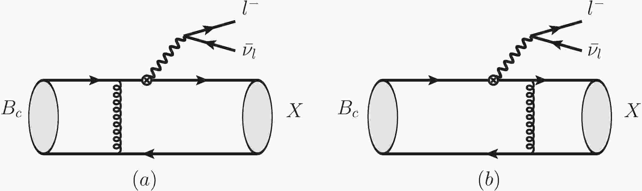
The lowest order Feynman diagrams for
$ B_c \to X l\nu $ are shown in Fig. 1. The kinematics of these decays is discussed in the large-recoil (low$ q^2 $ ) region, where the PQCD factorization approach is applicable to the semileptonic decays involving$ \eta_c $ or$ J/\psi $ as the final state meson, in Ref. [54]. In the rest frame of the$ B_c $ meson, we define the$ B_c $ meson momentum$ p_{1} $ , and the final state meson momentum$ p_{2} $ in the light-cone coordinates as [19, 55, 56]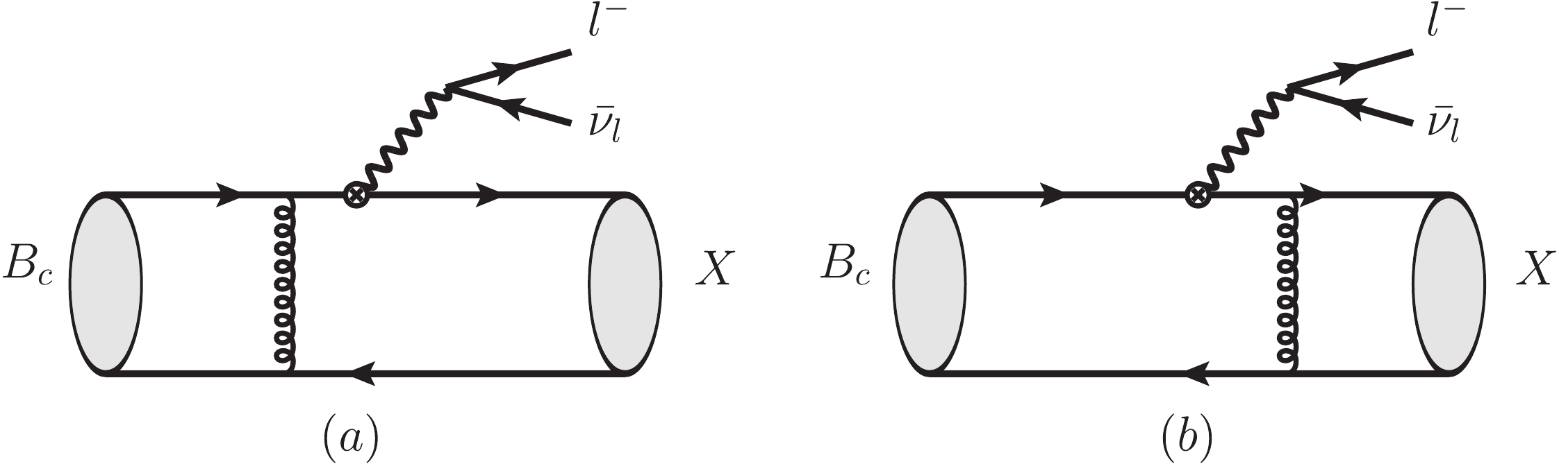
Figure 1. The charged current tree Feynman diagrams for the semileptonic decays
$ B_c^- \rightarrow (\eta_c, J/\psi) l^-\bar{\nu}_l $ with$ l = (e,\mu,\tau) $ in the PQCD approach.$ p_{\rm 1} = \frac{m_{ B_c}}{\sqrt{2}}(1,1,0_\bot),\quad p_{\rm 2} = r\frac{m_{ B_c}}{\sqrt{2}} (\eta^+,\eta^-,0_\bot), $

(6) with
$ \eta^{\pm} = \eta \pm \sqrt{\eta^2-1 }, \quad \eta = \frac{1}{2r}\left[ 1+ r^2-\frac{q^2}{ m_{B_c}^2 } \right], $

(7) where r is the mass ratio
$ r = m_{\eta_c}/m_{B_c} $ or$ m_{J/\psi}/m_{B_c} $ , and$ q = p_{\rm 1}-p_{\rm 2} $ is the momentum of the lepton pair. The longitudinal polarization vector$ \epsilon_{\rm L} $ and the transverse polarization vector$ \epsilon_{\rm T} $ of the vector meson are defined as in Ref. [19]:$ \epsilon_{\rm L} = \frac{1}{\sqrt{2}} (\eta^+,-\eta^-,0_\bot), \qquad \epsilon_{\rm T} = (0,0,1), $

(8) The momenta
$ k_1 $ and$ k_2 $ of the spectator quark in$ B_c $ , or in the final state$ (\eta_c,J/\psi) $ , are parametrized as in Ref. [19]:$ k_1 = \frac{m_{B_c}}{\sqrt{2}}(0,x_1,k_{1\bot}),\quad k_2 = \frac{r\cdot m_{B_c}}{\sqrt{2}}(x_2\eta^+,x_2\eta^-,k_{2\bot}), $

(9) where
$ x_{1,2} $ are the momentum fractions carried by the charm quark in the initial$ B_c $ and the final$ (\eta_c, J/\psi ) $ mesons.For the
$ B_c $ meson wave function, we make use of the example in Refs. [18, 19],$ \Phi_{B_c}(x,b) = \frac{\rm i}{\sqrt{6}} ({\not\!\! p}_1 +m_{B_c}) \gamma_5 \phi_{B_c} (x,b). $

(10) Here, we use the new DA
$ \phi_{B_c} (x,b) $ [51], as given in Eq. (4), instead of the simple$ \delta $ -function as in Eq. (5). As usual, the normalization constant$ N_{B_c} $ in Eq. (4) is given by the relation$ \int_0^1 \phi_{B_c}(x,b = 0){\rm d}x\equiv \int_0^1 \phi_{B_c}(x){\rm d}x = \frac{f_{B_c}}{2\sqrt{6}}, $

(11) where the decay constant
$ f_{B_c} = 0.489 \pm 0.005 $ GeV was obtained in lattice QCD by the TWQCD collaboration [57]. We set$ \beta_{B_c} = 1.0\pm 0.1 $ GeV in Eq. (4) in order to estimate the uncertainties [51].For the pseudoscalar charmonium state
$ \eta_c $ and the vector state$ J/\Psi $ , we use the same wave functions as in Refs. [19, 20]:$ \Phi_{\eta_c}(x) = \frac{\rm i}{\sqrt{6}}\gamma_5 \left [ {\not\!\! p} \phi^v(x)+m_{\eta_c}\phi^s(x) \right ], $

(12) $ \Phi_{J/\Psi}^L(x) = \frac{1}{\sqrt{6}} \left [ m_{J/\Psi} {\not\!\!\epsilon} _L \phi^L(x)+ {\not\!\!\epsilon} _L {\not\!\! p} \phi^{t}(x) \right ]\;, $

(13) $ \Phi_{J/\Psi}^T(x) = \frac{1}{\sqrt{6}} \left [ m_{J/\Psi} {\not\!\!\epsilon} _T \phi^V(x)+ {\not\!\!\epsilon} _T {\not \!\!p} \phi^{T}(x) \right ]\;, $

(14) where the twist-2 asymptotic DAs
$ (\phi^v(x),\phi^L(x),\phi^T(x)) $ , and the twist-3 DAs$ (\phi^s(x),\phi^t(x),\phi^V(x)) $ , are the same as in Refs. [19, 20]. -
For the charged current in the
$ B_c\to ( \eta_c,J/\psi ) l^-\bar{\nu}_l $ decays, the quark-level transition is the$ b\to c l^-\bar{\nu}_l $ decay with the effective Hamiltonian$ {\cal H}_{\rm eff}(b\to c l^-\bar{ \nu}_l) = \frac{G_{\rm F}}{\sqrt{2}}V_{cb}\; \bar{c} \gamma_{\mu}(1-\gamma_5)b \cdot \bar l\gamma^{\mu}(1-\gamma_5)\nu_l, $

(15) where
$ G_{\rm F} = 1.166 37\times10^{-5} \;{\rm{GeV}}^{-2} $ is the Fermi coupling constant, and$ V_{cb} $ is the CKM matrix element. The form factors$ f_{+,0}(q^2) $ of the$ B_c \to \eta_c $ transition are defined as in Refs. [55, 56, 58]:$\begin{split} \langle \eta_c (p_2)|\bar{c}(0)\gamma_{\mu}b(0)|B_c(p_1)\rangle = &\left[(p_1+p_2)_{\mu}-\frac{m_{B_c}^2-m_{\eta_c}^2}{q^2}q_{\mu}\right] f_+(q^2) \\& + \left[ \frac{m_{B_c}^2-m_{\eta_c}^2}{q^2}q_{\mu} \right] f_0(q^2). \end{split}$

(16) The differential decay widths of the semileptonic decays
$ B^-_c \to \eta_c l^-\bar{\nu}_{\rm l} $ can then be written [19, 22] in the following form:$ \begin{split} \frac{{\rm d}\Gamma(B_c \to \eta_c l\bar{\nu}_{\rm l})}{{\rm d}q^2} =& \frac{G_{\rm F}^2|V_{ cb}|^2}{192 \pi^3 m_{ B_c}^3} \left ( 1-\frac{m_{\rm l}^2}{q^2} \right)^2 \frac{\lambda^{1/2}(q^2)}{2q^2} \\& \times \Bigl \{ 3 m_{\rm l}^2\left (m_{ B_c}^2-m_{\rm \eta_c}^2 \right )^2 |f_{\rm 0}(q^2)|^2 \\&+ \left (m_{\rm l}^2+2q^2 \right )\lambda(q^2)|f_+(q^2)|^2 \Bigr \}, \end{split}$

(17) where
$ m_{\rm l} $ is the mass of the charged lepton,$ m_l^2 \leqslant q^2 \leqslant$ $ (m_{ B_c} -m_{\rm \eta_c})^2 $ , and$ \lambda(q^2) = (m_{ B_c}^2+m_{\rm \eta_c }^2-q^2)^2 - 4 m_{ B_c}^2 m_{\rm \eta_c }^2 $ is the phase space factor. In the PQCD factorization approach, the form factors$ f_0(q^2) $ and$ f_+(q^2) $ in Eqs. (16,17) are written as a sum of the auxiliary form factors$ f_{1,2}(q^2) $ :$ \begin{split} f_+(q^2) =& \frac{1}{2}\left [ f_1(q^2) + f_2(q^2)\right ], \\ f_0(q^2) = &f_{+}(q^2) + \frac{q^2}{2(m^2_{B_c} - m^2_{\eta_c})}\left [ f_1(q^2)- f_2(q^2) \right ] . \end{split}$

(18) After making the analytical calculations in the PQCD approach, the functions
$ f_{1,2}(q^2) $ are:$ \begin{split} f_1(q^2) =& 8\pi m_{B_c}^2C_{\rm F}\int {\rm d}x_1 {\rm d}x_2\int b_1 {\rm d}b_1 b_2 {\rm d}b_2 \;\phi_{B_c}(x_1,b_1)\\ &\times \Bigl\{\left[ -2r^2x_2 \phi^v(x_2)+2r(2-r_b)\phi^s(x_2) \right] \cdot H_1(t_1) \\ &+ \left[ \left ( -2r^2\!+\!\frac{rx_1\eta^+\eta^+}{\sqrt{\eta^2-1}} \right )\phi^v(x_2) \!+\!\left ( 4rr_c\!-\!\frac{2x_1r\eta^+}{\sqrt{\eta^2-1}} \right )\phi^s(x_2)\right] \\& \times H_2(t_2) \Bigr \}, \end{split} $

(19) $ \begin{split}f_2(q^2) = &8\pi m_{B_c}^2C_{\rm F}\int {\rm d}x_1 {\rm d}x_2\int b_1 {\rm d}b_1 b_2 {\rm d}b_2 \;\phi_{B_c}(x_1,b_1)\\& \times \Bigl\{ \left[(4r_b-2+4x_2r\eta)\phi^v(x_2)+(-4rx_2)\phi^s(x_2)\right] \cdot H_1(t_1) \\ &+ \left[ \left (-2r_c-\frac{x_1\eta^+}{\sqrt{\eta^2-1}} \right )\phi^v(x_2) +\left ( 4r+\frac{2x_1}{\sqrt{\eta^2-1}} \right )\phi^s(x_2)\right] \\& \times H_2(t_2) \Bigr \}, \end{split}$

(20) where the functions
$ H_i(t_i) $ are written in the following form$ H_i(t_i) = h_i(x_1,x_2,b_1,b_2) \cdot \alpha_s(t_i) \exp\left [-S_{ab}(t_i) \right ], \quad {\rm for} \ i = (1,2) , $

(21) and
$ C_{\rm F} = 4/3 $ is the color factor, and$ r_c = m_c/m_{B_c} $ ,$ r_b = m_b/m_{B_c} $ ,$ r = m_{\eta_c}/m_{B_c} $ . The symbol$ b_{i} $ in the above equations is the conjugate space coordinator of the transverse momentum$ k_{iT} $ . The symbol$ t_i $ in Eq. (21) represents the hard scale, chosen as the largest scale of virtuality of the internal particles in the hard$ b $ quark decay diagram,$ t_1 = \max\{\alpha_1, 1/b_1, 1/b_2\},\quad t_2 = \max\{\alpha_2, 1/b_1, 1/b_2\}. $

(22) The explicit expressions for the hard functions
$ h_i(x_1,x_2,b_1,b_2) $ and the Sudakov function$ \exp\left [-S_{ab}(t_i) \right ] $ are given in the Appendix.In the case of the final state vector meson
$ J/\psi $ , the form factors involved in the$ B_c \to J/\psi $ transition are$ V(q^2) $ and$ A_{0,1,2}(q^2) $ , defined in Refs. [55, 56, 58]$ \langle J/\psi (p_2)|\bar{c}(0) \gamma_{\mu} b(0)|B_c(p_1)\rangle = \frac{2{\rm i} V(q^2)}{m_{B_c}+m_{J/\psi}}\epsilon_{\mu \nu \alpha\beta} \epsilon^{* \nu}p_1^\alpha p_2^\beta, $

(23) $ \begin{split} \langle J/\psi(p_2)|\bar{c}(0) \gamma_{\mu}\gamma_5 b(0)|B_c(p_1)\rangle =& 2 m_{J/\psi}A_0(q^2)\frac{\epsilon^*\cdot q}{q^2}q_\mu + (m_{B_c} + m_{J/\psi})A_1(q^2) \left (\epsilon^*_\mu - \frac{\epsilon^*\cdot q}{q^2}q_\mu \right )\\& - A_2(q^2)\frac{\epsilon^*\cdot q}{m_{B_c} + m_{J/\psi}} \left [(p_1+p_2)_\mu - \frac{m_{B_c}^2-m_{J/\psi}^2}{q^2}q_\mu \right ]. \end{split} $

(24) The differential decay widths can be written in the following form [19, 22]:
$\begin{split} \frac{{\rm d}\Gamma_{\rm L}}{{\rm d}q^{\rm 2}} =& \frac{G_{\rm F}^{\rm 2}|V_{ cb}|^{\rm 2}}{192 \pi^3 m_{ B_c}^3} \left ( 1-\frac{m_{\rm l}^{\rm 2}}{q^{\rm 2}}\right )^{\rm 2} \frac{\lambda^{1/2}(q^{\rm 2})}{2q^{\rm 2}}\cdot \Bigg\{3m^{\rm 2}_{\rm l}\lambda(q^{\rm 2})A^{\rm 2}_{\rm 0}(q^{\rm 2})\\ & +\frac{m^{\rm 2}_{\rm l}+2q^{\rm 2}}{4m^{\rm 2}_{J/\psi }}\cdot \left [(m^{\rm 2}_{ B_c}-m^{\rm 2}_{J/\psi }-q^{\rm 2})(m_{ B_c}+m_{J/\psi}) A_{\rm 1}(q^{\rm 2}) -\frac{\lambda(q^{\rm 2})}{m_{ B_c}+m_{J/\psi }}A_{\rm 2}(q^{\rm 2}) \right ]^{\rm 2} \Bigg\}, \end{split} $

(25) $\begin{split} \frac{{\rm d}\Gamma_\pm}{{\rm d}q^{\rm 2}} =& \frac{G_{\rm F}^{\rm 2}|V_{ cb}|^{\rm 2}}{192 \pi^3 m_{ B_c}^3}\left ( 1-\frac{m_{\rm l}^{\rm 2}}{q^{\rm 2}}\right )^{\rm 2} \frac{\lambda^{3/2}(q^{\rm 2})}{2}\\& \times \left \{ (m^{\rm 2}_{\rm l}+2q^{\rm 2})\left[\frac{V(q^{\rm 2})}{m_{ B_c}+m_{J/\psi }}\mp \frac{(m_{ B_c}+m_{J/\psi })A_{\rm 1}(q^{\rm 2})}{\sqrt{\lambda(q^{\rm 2})}}\right]^{\rm 2}\right\}, \end{split}$

(26) where
$ m_l^2 \leqslant q^2 \leqslant (m_{ B_c} -m_{\rm J/\psi})^2 $ and$ \lambda(q^2) = (m_{ B_c}^2+m_{J/\psi }^2- $ $q^2)^2 - 4 m_{ B_c}^2 m_{J/\psi}^2 $ . The total differential decay width is defined as$ \frac{{\rm d}\Gamma}{{\rm d}q^{\rm 2}} = \frac{{\rm d}\Gamma_{\rm L}}{{\rm d}q^{\rm 2}} + \frac{{\rm d}\Gamma_+}{{\rm d}q^{\rm 2}} +\frac{{\rm d}\Gamma_-}{{\rm d}q^{\rm 2}}\; . $

(27) The form factors
$ V(q^2) $ and$ A_{0,1,2}(q^2) $ can also be calculated in the framework of the PQCD factorization approach:$ \begin{split} V(q^2) =& 8\pi m_{B_c}^2C_{\rm F}\int {\rm d}x_1 {\rm d}x_2\int b_1 {\rm d}b_1 b_2 {\rm d}b_2 \;\phi_{B_c}(x_1,b_1)\cdot (1+r)\\& \times \left \{\left[(2-r_b)\phi^T(x_2)-rx_2\phi^V(x_2)\right] \cdot H_1(t_1) + \left[\left(r+\frac{x_1}{2\sqrt{\eta^2-1}}\right)\phi^V(x_2) \right]\cdot H_2(t_2) \right \}, \end{split}$

(28) $\begin{split} A_0(q^2) =& 8\pi m_{B_c}^2C_{\rm F}\int {\rm d}x_1 {\rm d}x_2\int b_1 {\rm d}b_1 b_2 {\rm d}b_2 \;\phi_{B_c}(x_1,b_1) \times \Bigl \{ \left[\left(2r_b-1-r^2x_2+2rx_2\eta\right)\phi^L(x_2) +r\left(2-r_b-2x_2\right)\phi^t(x_2) \right] \cdot H_1(t_1) \\ &\left.+ \left [\left(r^2+r_c+\frac{x_1}{2}-rx_1\eta +\frac{x_1(\eta+r(1-2\eta^2))}{2\sqrt{\eta^2-1}} \right)\phi^L(x_2)\right ] \cdot H_2(t_2) \right \}, \end{split}$

(29) $ \begin{split} A_1(q^2) =& 8\pi m_{B_c}^2C_{\rm F}\int {\rm d}x_1 {\rm d}x_2\int b_1 {\rm d}b_1 b_2 {\rm d}b_2 \;\phi_{B_c}(x_1,b_1)\cdot \frac{r}{1+r} \times \Bigl \{\left [ 2(2r_b-1+rx_2\eta)\phi^V(x_2) -2(2rx_2-(2-r_b)\eta)\phi^T(x_2) \right ] \cdot H_1(t_1) \\ & + \left[ \left(2r_c-x_1+2r\eta \right) \phi^V(x_2)\right]\cdot H_2(t_2) \Bigr \}, \end{split}$

(30) $\begin{split} A_2(q^2) =& \frac{(1+r)^2(\eta-r)}{2r(\eta^2-1)}\cdot A_1(q^2)- 8\pi m_{B_c}^2C_{\rm F}\int {\rm d}x_1 {\rm d}x_2\int b_1 {\rm d}b_1 b_2 {\rm d}b_2 \;\phi_{B_c}(x_1,b_1)\cdot \frac{1+r}{\eta^2-1} \times \Bigg \{ \left[ \left [ 2x_2r(r-\eta)+(2-r_b)(1-r\eta) \right ]\phi^t(x_2) \right. \\& \left. + \left [ (1-2r_b)(r-\eta)-rx_2+2x_2r\eta^2-x_2r^2\eta \right ] \phi^L(x_2)\right] \cdot H_1(t_1) + \Bigg[ x_1\left(r\eta-\frac12\right)\sqrt{\eta^2-1} +\left(r_c-r^2-\frac{x_1}{2}\right)\eta \\&+r\left(1-r_c-\frac{x_1}{2}+x_1\eta^2\right) \Bigg] \cdot \phi^L(x_2) \cdot H_2(t_2) \Bigg\}, \end{split}$

(31) where
$ r_c = m_c/m_{B_c} $ ,$ r_b = m_b/m_{B_c} $ and$ r = m_{J/\psi}/m_{B_c} $ . The parameter$ \eta $ is defined in Eq. (7), and the functions$ H_i(t_i) $ are the same as those defined in Eq. (21). -
In the numerical calculations we used the following input parameters (masses and decay constants are in units of GeV) [1, 5, 15,58]:
$ \begin{split} m_{B_c} = &6.275,\quad m_{J/\psi} = 3.097,\quad m_{\tau} = 1.777, \\ m_{c} =& 1.27 \pm 0.03,\quad m_{\eta_c} = 2.983,\quad \tau_{B_c} = 0.507\; {\rm ps},\\ f_{ B_c} =& 0.489\pm 0.005, \quad f_{\eta_c} = 0.438\pm 0.008, \\ f_{J/\psi} =& 0.405 \pm 0.014, \quad |V_{cb}| =(42.2 \pm 0.8)\times 10^{-3}, \\ \Lambda^{ (f = 4)}_{\overline{\rm MS}} =& 0.287. \end{split}$

(32) In the case of semileptonic
$ B_c $ meson decays, it is easy to see that the theoretical predictions of the differential decay rates and other physical observables strongly depend on the form factors$ f_{\rm 0,+}(q^{\rm 2}) $ for the$ B_c \to \eta_c l \nu_l $ decays, and the form factors$ V(q^{\rm 2}) $ and$ A_{\rm 0,1,2}(q^{\rm 2}) $ for the$ B_c \to J/\psi l \nu_l $ decays [19, 22]. The value of these form factors at$ q^2 = 0 $ and their$ q^2 $ dependence in the whole range of$ 0\leqslant q^2 \leqslant q^2_{\max} $ contain a lot of information about the physical process. These form factors have been calculated using different methods, for example, in Refs. [21, 25, 26, 28, 29, 31, 33].In Refs. [7, 8, 56, 59], the applicability of the PQCD factorization approach to the
$ (B \to D^{(*)}) $ transitions was examined, and it was shown that the PQCD approach with the inclusion of the Sudakov effects is applicable to the study of semileptonic decays$ B \to D^{(*)} l\bar{\nu}_{\rm l} $ [7, 8]. Since the PQCD predictions of the form factors are reliable only in the low$ q^{\rm 2} $ region, we first calculate explicitly the values of the relevant form factors at sixteen points in the region$ 0 \leqslant q^{\rm 2}\leqslant m_{\rm \tau}^{\rm 2} $ using the expressions given in Eqs. (19, 20, 28-31) and the definitions in Eq. (18). In the second column of Table 1, we show the PQCD predictions of the six relevant form factors at$ q^2 = 0 $ . The errors of the PQCD predictions are a combination of the uncertainties of$ \beta_{ B_c} = 1.0\pm 0.1 $ GeV,$ m_{ c} = 1.27 \pm 0.03 $ GeV and$ |V_{cb}| = $ $ (42.2 \pm 0.8)\times 10^{-3} $ . In the third column of Table 1, we show the previous PQCD predictions presented in Ref. [19]. As a comparison, we also list the central values of the form factors$ f_i(0) $ obtained by other approaches, such as BSW [60], NRQCD [39], LCSR [21, 32], RQM and CCQM methods [26, 35], and the lattice QCD [44].form factors PQCD This work PQCD [19] LFQM [22] BSW [60] NRQCD [39] LCSR [21] LCSR [32] RQM [26] CCQM [35] lattice [44] $ f_{\rm 0,+} ^{B_c\to \eta_c}(0)$ 

0.56(7) 0.48(7) 0.61 0.58 1.67 0.87 0.62 0.47 0.75 0.59 $ V ^{ {B_c}\to {{J} }/\psi}(0)$ 

0.75(9) 0.42(2) 0.74 0.91 2.24 1.69 0.73 0.49 0.78 0.70 $ A_{\rm 0} ^{ {B_c}\to {{J} }/\psi}(0)$ 

0.40(5) 0.59(3) 0.53 0.58 1.43 0.27 0.54 0.40 0.56 − $ A_{\rm 1}^{ {B_c}\to {{J} }/\psi} (0)$ 

0.47(5) 0.46(3) 0.50 0.63 1.57 0.75 0.55 0.73 0.55 0.48 $ A_{\rm 2}^{ {B_c}\to {{J} }/\psi} (0)$ 

0.62(6) 0.64(3) 0.44 0.74 1.73 1.69 0.35 0.50 0.56 − It is easy to see from the numerical values given in Table 1 that: (a) the PQCD predictions of
$ f_{0,+}(0) $ ,$ V(0) $ and$ A_1(0) $ agree very well with the corresponding lattice QCD results, and (b) that the predictions of different approaches can vary by large factors, for instance, by a factor of three for$ f_{0,+}(0) $ . Since the PQCD calculations of the form factors are not reliable for large$ q^{\rm 2} $ , we have to make an extrapolation from the low$ q^{\rm 2} $ to the large$ q^{\rm 2} $ regions. In this work, we make the extrapolation using the following two methods.In the first method, we use our PQCD predictions of all relevant form factors
$ f_i(q^2) $ at sixteen points in$ 0\leqslant q^2 \leqslant m^2_\tau $ as input, and make the extrapolation from the low$ q^2 $ region to$ q_{\rm max}^2 $ using the Bourrely-Caprini-Lellouch (BCL) parametrization [52]. Similarly to Ref. [32], we consider only the first two terms of the series in the parameter$ z $ :$\begin{split} f_i(t) =& \frac{1}{1-t/m^2_R} \sum\limits_{k = 0}^{1} \alpha^i_k\; z^k(t,t_0)\\ =& \frac{1}{1-t/m^2_R} \left ( \alpha^i_0 + \alpha^i_1\; \frac{ \sqrt{t_+ - t} - \sqrt{t_+ - t_0}}{\sqrt{t_+ - t} + \sqrt{t_+ - t_0}} \right ) , \end{split}$

(33) where
$ t = q^2 $ ,$ m_R $ are the masses of the low-lying$ B_c $ resonances listed in Table 2, and the parameters$ t_\pm $ and$ t_0 $ are the same ones as being defined in Refs. [32, 61]:FFs $ f_i(0) $ in PQCD

$ J^P $ 

$ m_R $ 

$ \alpha_0 $ 

$ \alpha_1 $ 

$ f_0 $ 

0.56(7) $ 0^+ $ 

6.71 0.691 −7.74 $ f_+ $ 

0.56(7) $ 1^- $ 

6.34 0.763 −12.2 $ V $ 

0.75(9) $ 1^- $ 

6.34 1.06 −20.6 $ A_0 $ 

0.40(5) $ 0^- $ 

6.28 0.551 −10.5 $ A_1 $ 

0.47(5) $ 1^+ $ 

6.75 0.586 −7.73 $ A_2 $ 

0.62(6) $ 1^+ $ 

6.75 1.01 −26.8 Table 2. Form factors
$ f_i(0) $ obtained from the PQCD calculations,$ J^P $ and masses (in units of GeV) of the low-lying$ B_c $ resonances [32] used in the BCL fit of the$ B_c \to (\eta_c,J/\psi) $ form factors. The parameters$ \alpha_{0,1} $ are determined from the fit.$ 0 \leqslant t_{0} = t_+ \left (1 - \sqrt{1 - \frac{t_-}{t_+}} \right ) \leqslant t_-, \\ t_{\pm} = (m_{B_c} \pm m_x)^2 , $

(34) where
$ m_x = m_{\eta_c} $ or$ m_{J/\psi} $ for the$ B_c \to \eta_c $ or$ J/\psi $ transitions, respectively. In Table 2, we list the PQCD input:$ f_i(0) $ , the masses$ m_R $ , parameters$ \alpha_0 $ and$ \alpha_1 $ determined from the BCL fitting procedure for$ B_c \to \eta_c $ , and the$ B_c \to J/\psi $ form factors. The values of$ m_R $ are taken from Ref. [32].The second method is the “PQCD+Lattice” method, similar to what we did in Ref. [62] for the studies of
$ R(D^{*}) $ . As mentioned in the Introduction, the HPQCD collaboration [44, 45] calculated the form factors$ f_{0,+}(q^2) $ for the$ B_c \to \eta_c $ transition, and$ V(q^2) $ and$ A_1(q^2) $ for the$ B_c \to J/\psi $ transition using the lattice QCD method (working directly at$ m_b $ with an improved NRQCD effective theory formulism) at$ q^2 = 0 $ and several other values of$ q^2 $ . In order to improve the reliability of the extrapolation of$ f_i(q^2) $ to the large$ q^2 $ region, we use the currently available "Lattice'' results for$ q^2 = (5.44, 8.72,10.07) $ GeV2 , as given in Refs. [44, 45],$ \begin{split} f_0(8.72) =& 0.823\pm 0.050, \quad f_+(8.72) = 0.995\pm 0.050, \\ V(5.44) =& 1.06\pm 0.05, \quad A_1(10.07) = 0.788\pm 0.050, \end{split}$

(35) as the lattice QCD input for fitting of the form factors
$ (f_{0,+}(q^2), V(q^2), A_1(q^2)) $ using the BCL parametrization [52]. In order to estimate the effect of possible uncertainties of the lattice QCD input, we assume a five percent error ($ \pm 0.05 $ ) of the four form factors in Eq. (35). For the other two form factors,$ A_{0}(q^2) $ and$ A_{2}(q^2) $ , there are no lattice QCD results available at present.In Figs. 2 and 3, we show the theoretical predictions of the
$ q^2 $ dependence of the six form factors relevant for the$ B_c \to (\eta_c,J/\psi) $ transitions, obtained using the PQCD approach and the “PQCD+Lattice” approach. In these figures, the blue solid curves indicate the theoretical predictions of the$ q^2 $ dependence of$ f_{0,+}(q^2) $ ,$ V(q^2) $ and$ A_{0,1,2}(q^2) $ in the PQCD approach, while the red dashed curves indicate the four form factors$ (f_{0,+}(q^2), $ $ V(q^2), A_1(q^2)) $ obtained by the “PQCD+Lattice” approach. The bands in the figures are the uncertainties of the corresponding theoretical predictions. The four black dots in Figs. 2 and 3 are the lattice QCD input in Eq. (35) used in the fitting procedure. One can see from the theoretical predictions shown in Figs. 2 and 3 that the form factors and their$ q^2 $ dependence obtained using the two methods agree very well in the whole range of$ q^2 $ .
Figure 2. (color online) Theoretical predictions of the
$ B_c \to \eta_c $ transition form factors$ f_+(q^2) $ and$ f_0(q^2) $ in the PQCD approach (blue solid curve), and in the "PQCD+Lattice" approach (red dashed curve). The large dots are the lattice QCD input given in Eq. (35).
Figure 3. (color online) Theoretical predictions of the
$ B_c \to J/\psi $ transition form factors$ V(q^2) $ and$ A_{0,1,2}(q^2) $ in the PQCD approach (blue solid curve), and in the "PQCD+Lattice" approach (red dashed curve). The large dots in (a,c) are the lattice QCD input given in Eq. (35).In Fig. 4, we show the
$ q^2 $ dependence of the theoretical predictions of the differential decay rates$ {\rm d}\Gamma /{\rm d}q^2 $ for the semileptonic decays$ B_c \to (\eta_c,J/\psi) l \bar{\nu}_l $ with$ l = (\mu,\tau) $ , where the blue solid curve and the red dashed curve indicate$ {\rm d}\Gamma /{\rm d}q^2 $ in the PQCD approach and “PQCD+Lattice” method, respectively. For the four$ B_c \to $ $ (\eta_c,J/\psi)( \mu^- \bar{\nu}_{\mu},\tau^-\bar{\nu}_{\tau} ) $ decays considered, the theoretical predictions of the differential decay rates with the two approaches agree well within the errors in the whole$ q^2 $ region. For the$ B_c \to J/\psi \mu^- \bar{\nu}_{\mu} $ decay, on the other hand, a difference between the central values can be seen in the large$ q^2 $ region, but remains small in size. We hope that the lattice results for the form factors$ A_{0,2}(q^2) $ will become available soon, which may help to improve our results.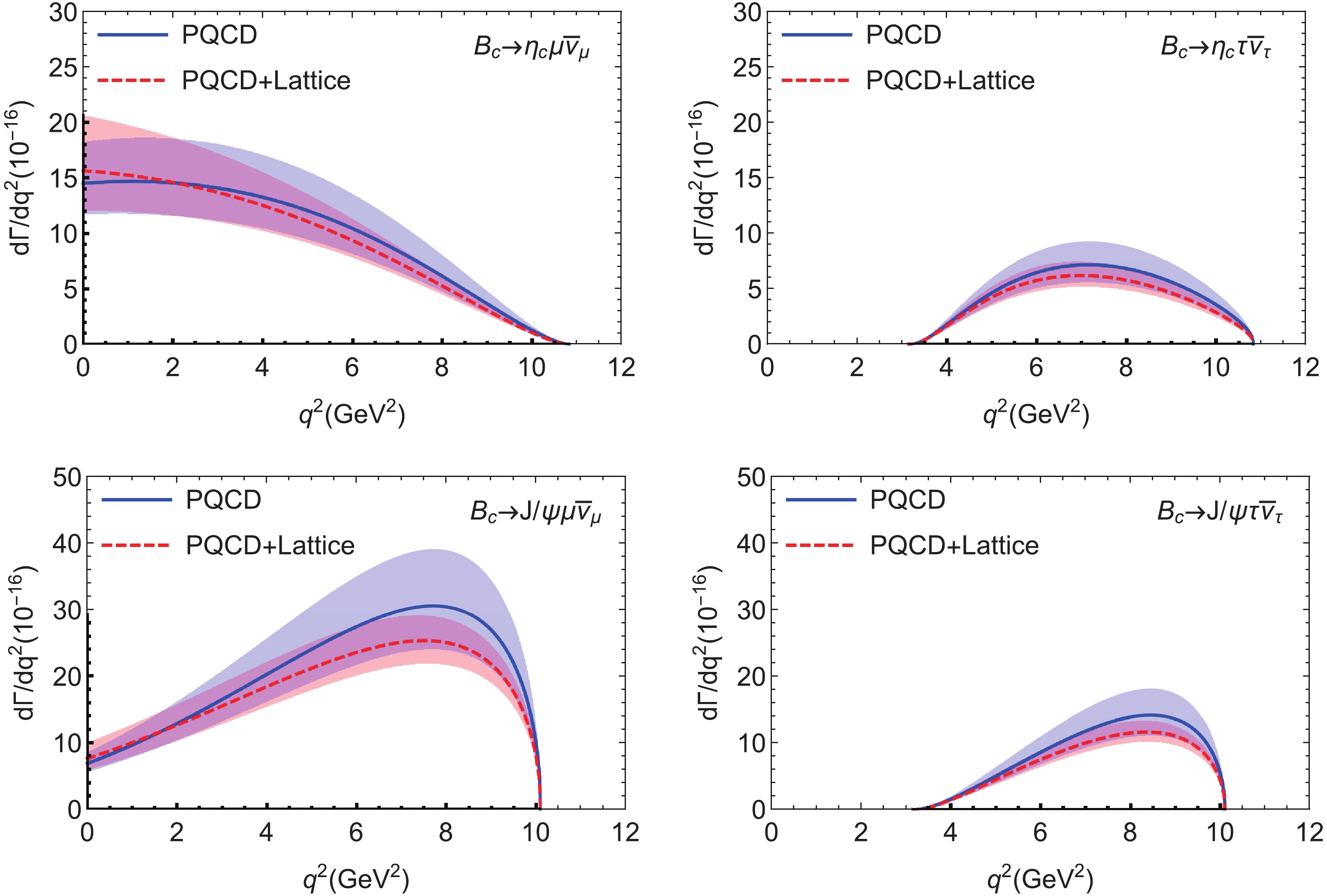
Figure 4. (color online) Theoretical predictions of the
$ q^2 $ dependence of$ {\rm d}\Gamma /{\rm d}q^2 $ for the decays$ B_c \to (\eta_c,J/\psi) (\mu \bar{\nu}_{\mu}, \tau \bar{\nu}_{\tau}) $ in the PQCD and “PQCD+Lattice” approaches. The bands show the theoretical uncertainties.From the formulae for the differential decay rates in Eqs. (17,27), it is straightforward to make an integration over the range
$ m^2_l \leqslant q^2 \leqslant (m^2_{B_c} - m_x^2) $ with$ x = (\eta_c,J/\psi) $ . The theoretical predictions (in units of$ 10^{-3} $ ) for the branching ratios of the semileptonic decays considered are the following:$ {\cal B}(B_c \to \eta_c \tau \bar{\nu}_\tau) = \left \{ \begin{array}{ll} 2.79^{+0.83}_{-0.61}(\beta_{ B_c}) \pm 0.11(V_{ cb}) \pm 0.09 (m_{ c}) , & {\rm PQCD}, \\ 2.41^{+0.48}_{-0.39}(\beta_{ B_c})\pm 0.09(V_{ cb}) \pm 0.04 (m_{\rm c}) , & {\rm PQCD+Lattice}, \end{array} \right. $

(36) $ {\cal B}(B_c \to \eta_c \mu \bar{\nu}_\mu ) = \left \{ \begin{array}{ll} 8.14^{+1.91}_{-1.72}(\beta_{ B_c}) \pm 0.31(V_{ cb}) \pm 0.30 (m_{ c}) , & {\rm PQCD}, \\ 7.76^{+1.92}_{-1.46}(\beta_{B_c})\pm 0.29(V_{ cb}) \pm 0.24 (m_{ c}) , & {\rm PQCD+Lattice}, \\ \end{array} \right. $

(37) $ {\cal B}(B_c \to J/\psi \tau \bar{\nu}_{\tau}) = \left \{ \begin{array}{ll} 4.54^{+1.27}_{-0.98}(\beta_{ B_c})\pm 0.18(V_{ cb}) \pm 0.16 (m_{ c}) , & {\rm PQCD}, \\ 3.83^{+0.61}_{-0.55}(\beta_{ B_c})\pm 0.14(V_{ cb}) \pm 0.10 (m_{ c}) , & {\rm PQCD+Lattice}, \\ \end{array} \right. $

(38) $ {\cal B}(B_c \to J/\psi \mu \bar{\nu}_{\mu}) = \left \{ \begin{array}{ll} 16.1^{+4.4}_{-3.3}(\beta_{ B_c})\pm 0.61 (V_{ cb}) \pm 0.52 (m_{ c}) , & {\rm PQCD}, \\ 14.1^{+2.6}_{-2.1}(\beta_{ B_c})\pm 0.51(V_{ cb}) \pm 0.36 (m_{ c}) , & {\rm PQCD+Lattice}, \\ \end{array} \right. $

(39) where the dominant errors come from the uncertainties of the input parameters
$ \beta_{ B_c} = 1.0\pm 0.1 $ GeV,$ |V_{ cb}| = (42.2\pm $ $0.8) \times 10^{-3} $ and$ m_{ c} = 1.27\pm 0.03 $ GeV.In Table 3, we list the theoretical predictions (in units of
$ 10^{-3} $ ) of the branching ratios of the decays$ B_c \to (\eta_c,J/\psi ) l^- \bar{\nu}_l $ with$ l = (\mu,\tau) $ , obtained using the PQCD and "PQCD+Lattice" approaches. As a comparison, we also show the results from our previous PQCD work [19], and from several other models or approaches [21, 22, 32, 43]. One can see that the difference between the theoretical predictions can be as large as a factor of two for the same decay mode. In Table 4, we show our theoretical predictions of the ratios$ R_{\eta_c} $ and$ R_{J/\psi} $ , defined in Eq. (1). Previous results given in Refs. [19, 21, 22, 32, 40, 41, 43] are also listed for comparison. The measured value of$ R_{J/\psi} = 0.71 \pm 0.24 $ by the LHCb collaboration [17] is listed in the last column of Table 4.mode PQCD PQCD+Lattice PQCD [19] LFQM [22] Z-Series [43] LCSR [21] LCSR [32] $ {\cal B}(B_c \to \eta_c\mu \bar{\nu}_\mu) $ 

$ 8.14^{+1.96}_{-1.77} $ 

$ 7.76^{+1.95}_{-1.51} $ 

$ 4.4^{+1.2}_{-1.1} $ 

6.7 6.6 16.7 $ 8.2^{+1.2}_{-1.1} $ 

$ {\cal B}(B_c \to \eta_c\tau \bar{\nu}_\tau) $ 

$ 2.79^{+0.84}_{-0.63} $ 

$ 2.41^{+0.49}_{-0.40} $ 

$ 1.4^{+0.4}_{-0.3} $ 

1.9 2.0 4.9 $ 2.6^{+0.6}_{-0.5} $ 

$ {\cal B}(B_c \to J/\psi \mu \bar{\nu}_\mu) $ 

$ 16.1^{+4.5}_{-3.4} $ 

$ 14.1^{+2.7}_{-2.2} $ 

$ 10.0^{+1.3}_{-1.2} $ 

14.9 14.5 23.7 $ 22.4^{+5.7}_{-4.9} $ 

$ {\cal B}(B_c \to J/\psi\tau \bar{\nu}_\tau ) $ 

$ 4.54^{+1.29}_{-1.01} $ 

$ 3.83^{+0.63}_{-0.58} $ 

$ 2.9 ^{+0.4}_{-0.3} $ 

3.7 3.6 6.5 $ 5.3^{+1.6}_{-1.4} $ 

Table 3. Theoretical predictions (in units of
$ 10^{-3} $ ) of the branching ratios$ {\cal B}(B_c \to (\eta_c,J/\psi ) l \bar{\nu}_l) $ obtained using the PQCD and "PQCD+Lattice" approaches. As a comparison, the predictions in the previous PQCD work [19], and other four approaches [21, 22, 32, 43], are also given.From the theoretical predictions of the branching ratios and of the ratios
$ R_{\eta_c} $ and$ R_{J/\psi} $ given in Eqs. (36-39) and Tables 3 and 4, we find the following points:(1) The theoretical predictions of the branching ratios of all
$ B_c \to (\eta_c,J/\psi ) l^- \bar{\nu}_l $ decays considered using the PQCD and “PQCD+Lattice” approaches agree well within the errors (around 30% in magnitude). Numerically, the theoretical predictions for a given decay mode becomes smaller by about 5%-16% when the lattice QCD results for the form factors$ (f_{0,+},V, A_1) $ are taken into account in the extrapolation of the relevant form factors to the high$ q^2 $ region.(2) The theoretical predictions of the ratios
$ R_{\eta_c} $ and$ R_{J/\psi} $ in the PQCD and “PQCD+Lattice” approaches agree very well, and have small errors (less than 5% in magnitude) due to the strong cancellation between the errors of the branching ratios. Although the theoretical predictions of$ R_{J/\psi} $ listed in Table 4 are smaller in both the PQCD and “PQCD+Lattice” approaches than the measured value$ 0.71\pm 0.24 $ reported by the LHCb collaboration [17], they may be considered to agree because of the relatively large error of the experimental measurement. We believe that the ratios$ R_{\eta_c} $ and$ R_{J/\psi} $ could be measured to a higher precision by the LHCb experiment in the future, which would help to test the theoretical models or approaches.(3) Although the theoretical predictions of the decay rates using different methods or approaches can be rather different, even by a factor of two or three, the theoretical predictions of the ratios
$ R_{\eta_c} $ and$ R_{J/\psi} $ in different works [19, 21, 22, 32, 39, 43] agree very well within 30% of the central value.In both kinds of semileptonic decays
$ B \to D^{(*)} l^- \bar{\nu}_l $ and$ B_c^- \to (\eta_c,J/\psi ) l^- \bar{\nu}_l $ , the quark level weak decays are the same charged current tree transitions:$ b \to c l^- \bar{\nu}_l $ with$ l = (e,\mu,\tau) $ . The only difference between them is the spectator quark: in the first case it is the heavy charm quark, while in the second it is the light up or down quark. As a consequence, it is reasonable to assume that the dynamics of these semileptonic decays is similar, and we can therefore use a similar method to study these semileptonic decays.For the
$ B \to D^{(*)} \tau \bar{\nu}_\tau $ decay, besides the decay rate and the ratio$ R( D^{(*)}) $ , the longitudinal polarization$ P_{\tau}(D^{(*)}) $ of the tau lepton and the fraction of$ D^* $ longitudinal polarization$ F_L^{D^*} $ are also additional physical observables sensitive to new physics [63-66]. The first measurement of$ P_\tau(D^*) $ and$ F_L^{D^*} $ was reported recently by the Belle collaboration [53, 67, 68]:$ P_\tau( D^*) = -0.38 \pm 0.51({\rm stat.}) ^{+0.21}_{-0.16}({\rm syst.}), $

(40) $ F_L(D^*) = 0.60 \pm 0.08({\rm stat.}) \pm 0.04 ({\rm syst.}). $

(41) These values are compatible with the SM predictions:
$P_\tau( D^*) = $ $ -0.497 \pm 0.013 $ for$ \bar{B} \to D^* \tau^- \bar{\nu}_\tau $ [64, 66], and$ F_L(D^*) = $ $0.441 \pm 0.006 $ [69] or$ 0.457\pm 0.010 $ [70].For the
$ B_c \to (\eta_c,J/\psi) \tau \bar{\nu}_\tau $ decay, we consider the relevant longitudinal polarizations$ P_\tau(\eta_c) $ and$ P_\tau(J/\psi) $ , and define them in the same way as$ P_\tau(D^{(*)}) $ in Refs. [63-66]:$ P_\tau(X) = \frac{\Gamma^+(X) - \Gamma^-(X)}{ \Gamma^+(X) + \Gamma^-(X) }, \quad {\rm for} \quad X = (\eta_c,J/\psi), $

(42) where
$ \Gamma^\pm(X) $ denotes the decay rates of$ B_c\to X \tau \bar{\nu}_\tau $ with$ \tau $ lepton helicity$ \pm 1/2 $ . Following Ref. [65], the explicit expressions for$ {\rm d}\Gamma^\pm/{\rm d}q^2 $ and the semileptonic$ B_c $ decays considered here can be written in the following form:$ \begin{split} \frac{{\rm d}\Gamma^{+} }{{\rm d}q^2} (B_c \to \eta_c \tau \bar{ \nu}_{\tau} ) =& \frac{ G_{\rm F}^2 |V_{cb}|^2}{ 192\pi^3 m_{B_c}^3} \; q^2 \sqrt{\lambda(q^2)} \left( 1 - \frac{m_\tau^2}{ q^2} \right)^2\\&\times \frac{m_\tau^2}{ 2q^2} \left ( H_{V,0}^{s\,2} + 3 H_{V,t}^{s\,2} \right) , \end{split} $

(43) $\frac{{{\rm d}{\Gamma ^ - }}}{{{\rm d}{q^2}}}({B_c} \to {\eta _c}\tau {\bar \nu _\tau }) = \frac{{G_{\rm F}^2|{V_{cb}}{|^2}}}{{192{\pi ^3}m_{{B_c}}^3\;}}{q^2}\sqrt {\lambda ({q^2})} {\left( {1 - \frac{{m_\tau ^2}}{{{q^2}}}} \right)^2}\left( {H_{V,0}^{s{\kern 1pt} 2}} \right),$

(44) $\begin{split} \frac{{{\rm d}{\Gamma ^ + }}}{{{\rm d}{q^2}}}({B_c} \to J/\psi \tau {{\bar \nu }_\tau }) =& \frac{{G_{\rm F}^2|{V_{cb}}{|^2}}}{{192{\pi ^3}m_{{B_c}}^3}}\;{q^2}\sqrt {\lambda ({q^2})} {\left( {1 - \frac{{m_\tau ^2}}{{{q^2}}}} \right)^2}\frac{{m_\tau ^2}}{{2{q^2}}}\\ &\times \left( {H_{V, + }^2 + H_{V, - }^2 + H_{V,0}^2 + 3H_{V,t}^2} \right), \end{split}$

(45) $\begin{split}\frac{{{\rm d}{\Gamma ^ - }}}{{{\rm d}{q^2}}}({B_c} \to J/\psi \tau {\bar \nu _\tau }) =& \frac{{G_{\rm F}^2|{V_{cb}}{|^2}}}{{192{\pi ^3}m_{{B_c}}^3}}\;{q^2}\sqrt {\lambda ({q^2})} {\left( {1 - \frac{{m_\tau ^2}}{{{q^2}}}} \right)^2}\\&\times\left( {H_{V, + }^2 + H_{V, - }^2 + H_{V,0}^2} \right),\end{split}$

(46) with the functions
$ H_i(q^2) $ $H_{V,0}^s({q^2}) = \sqrt {\frac{{\lambda ({q^2})}}{{{q^2}}}} {f_ + }({q^2}),$

(47) $H_{V,t}^s({q^2}) = \frac{{m_{{B_c}}^2 - m_{{\eta _c}}^2}}{{\sqrt {{q^2}} }}{f_0}({q^2}), $

(48) $ {H_{V, \pm }}({q^2}) = ({m_{{B_c}}} + {m_{J/\psi }}){A_1}({q^2}) \mp \frac{{\sqrt {\lambda ({q^2})} \;V({q^2})}}{{{m_{{B_c}}} + {m_{J/\psi }}}}, $

(49) $\begin{split} {H_{V,0}}({q^2}) =& \frac{{{m_{{B_c}}} + {m_{J/\psi }}}}{{2{m_{J/\psi }}\sqrt {{q^2}} }}\bigg[ { - (m_{{B_c}}^2 - m_{J/\psi }^2 - {q^2}){A_1}({q^2})} \\&\left.+ \frac{{\lambda ({q^2})\;{A_2}({q^2})}}{{{{({m_{{B_c}}} + {m_{J/\psi }})}^2}}} \right], \end{split}$

(50) $ {H_{V,t}}({q^2}) = - \sqrt {\frac{{\lambda ({q^2})}}{{{q^2}}}} {A_0}({q^2}), $

(51) where
$ m_l^2 \leqslant q^2 \leqslant \left (m_{\rm B_c} -m_X \right )^2 $ and$ \lambda(q^2) = \left ( m_{\rm B_c}^2+m_X^2-q^2 \right )^2 - $ $4 m_{ B_c}^2 m_X^2 $ with$ X = (\eta_c,J/\psi) $ , and the explicit expressions for the form factors$ f_{+,0}(q^2) $ ,$ V(q^2) $ and$ A_{0,1,2}(q^2) $ in the PQCD approach are given in Eqs. (18), (28)-(31).After making the proper integrations over
$ q^2 $ , we find the following theoretical predictions of the longitudinal polarization$ P_\tau $ in the semileptonic$B_c \!\!\to $ $ (\eta_c,J/\psi) l^- \bar{\nu}_l $ decays:$ P_{\tau}( \eta_c) = 0.37\pm 0.01, \quad P_{\tau}(J/\psi) = -0.55 \pm 0.01, $

(52) in the PQCD approach, and
$ P_{\tau}(\eta_c) = 0.36\pm 0.01, \qquad P_{\tau}(J/\psi) = -0.53\pm 0.01 , $

(53) in the “PQCD+Lattice” approach. The dominant errors come from the uncertainty of
$ \beta_{B_c} $ and$ m_c $ . Following the measurement of the longitudinal polarization$ P_{\tau}(D^*) $ for$ B \to D^* \tau \nu_\tau $ by Belle [53], we believe that similar measurements of the longitudinal polarizations$ P_{\tau}(\eta_c) $ and$ P_{\tau}( J/\psi) $ could be made by the LHCb experiment in the near future, when a sufficient number of$ B_c $ decay events is collected. -
We studied the semileptonic decays
$ B_c \to (\eta_c,J/\psi) l \bar{\nu} $ using the PQCD factorization approach with new input: (a) we used the newly defined DAs of the$ B_c $ meson instead of the delta function; (b) the new BCL parametrization for extrapolating the form factors from the low$ q^2 $ region to$ q^2_{\max} $ ; and (c) we have taken into account the current lattice QCD results for the form factors as new input in our fitting procedure. We calculated the form factors$ f_{\rm 0,+}(q^{\rm 2}) $ ,$ V(q^{\rm 2}) $ and$ A_{\rm 0,1,2}(q^{\rm 2}) $ of the$ B_c \to (\eta_c,J/\psi) $ transitions, presented the predictions for the branching ratios$ {\cal B}(B_c \to (\eta_c,J/\psi) l \bar{\nu}_l) $ , the ratios$ R_{\eta_c} $ and$ R_{J/\psi} $ of the branching ratios, and the longitudinal polarizations$ P_\tau(\eta_c) $ and$ P_\tau(J/\psi) $ of the final$ \tau $ lepton.From the numerical calculations and phenomenological analysis we found the following:
(1) The theoretical predictions of the branching ratios of the
$ B_c \to (\eta_c,J/\psi) l \bar{\nu} $ decays with the PQCD and “PQCD+Lattice” approaches agree very well. A small decrease of about 5%-16% is introduced when the lattice QCD input for the form factors$ (f_{0,+}(8.72),V(5.44), $ $A_1(10.07)) $ is taken into account in the extrapolation of the form factors to the high$ q^2 $ region.(2) The theoretical predictions of the ratios
$ R_{\eta_c} $ and$ R_{J/\psi} $ are the following:$ R_{\rm \eta_c} = 0.34\pm 0.01, \quad R_{ J/\psi} = 0.28\pm 0.01, \quad {\rm in \;\; PQCD}, $

(54) $ R_{\rm \eta_c} = 0.31\pm 0.01 , \quad R_{ J/\psi} = 0.27\pm 0.01, \quad {\rm in \;\; PQCD+Lattice}. $

(55) The central values of the above predictions of
$ R_{J/\psi} $ are smaller than the measured values, as shown in Eq. (2), but still agree within the errors.(3) The theoretical predictions of the longitudinal polarization
$ P(\tau) $ of the tau lepton are the following:$\begin{split} P_{\tau}( \eta_c) =& 0.37\pm 0.01, \\ P_{\tau}(J/\psi) =& -0.55 \pm 0.01, \quad {\rm in \; \; PQCD}, \end{split}$

(56) $\begin{split} P_{\tau}( \eta_c) = &0.36\pm 0.01, \\ P_{\tau}(J/\psi) =& -0.53\pm 0.01 , \quad{\rm in \; PQCD+Lattice}. \end{split}$

(57) These predictions could be tested by the LHCb experiment in the near future.
We wish to thank Wen-Fei Wang and Ying-Ying Fan for valuable discussions.
-
In this Appendix, we present explicit expressions for some functions that appeared in the previous sections. The hard functions
$ h_{1,2}(x_1,x_2b_1,b_2) $ in Eq. (21) can be written as$\tag{A1} \begin{split}h_1 =& K_0(\beta_1 b_1) \left [ \theta(b_1-b_2)I_0(\alpha_1b_2)K_0(\alpha_1b_1)\right. \\&\left.+\theta(b_2-b_1)I_0(\alpha_1b_1)K_0(\alpha_1b_2) \right ], \\ h_2 =& K_0(\beta_2 b_2) \left [\theta(b_1-b_2)I_0(\alpha_2b_2)K_0(\alpha_2b_1)\right. \\&\left.+\theta(b_2-b_1)I_0(\alpha_2b_1)K_0(\alpha_2b_2) \right ], \end{split} $

with
$ \tag{A2} \begin{split}\alpha_1 =& m_{B_c}\sqrt{2rx_2\eta+r^2_b-1-r^2x^2_2} , \\ \alpha_2 =& m_{B_c}\sqrt{rx_1\eta^++r^2_c-r^2} , \\ \beta_1 =& \beta_2 = m_{B_c}\sqrt{x_1x_2r\eta^+-r^2x^2_2}, \end{split} $

where
$ r_q = m_q/m_{B_c} $ with$ q = (c,b) $ ,$ r = m_{\eta_c}/m_{B_c} $ ($ r = m_{J/\psi}/m_{B_c} $ ) when it appears in the form factors$ f_{+,0}(q^2) $ ($ V(q^2) $ and$ A_{0,1,2}(q^2) $ ).$ \eta $ and$ \eta^+ $ are defined in Eq. (7). The functions$ K_0 $ and$ I_0 $ in Eq. (A1) are the modified Bessel functions. The term inside the square-root of$ \alpha_{(1,2)} $ and$ \beta_{(1,2)} $ may be positive or negative. When this term is negative, the argument of the functions$ K_0 $ and$ I_0 $ is imaginary, and the associated Bessel functions$ K_0 $ and$ I_0 $ transform in the following way$ \tag{A3}\begin{split} K_0(\sqrt{y})|_{y<0} = &K_0({\rm i} \sqrt{|y|}) = \frac{{\rm i} \pi}{2} [J_0(\sqrt{|y|}) + {\rm i} Y_0(\sqrt{|y|})] \\ I_0(\sqrt{y})|_{y<0} =& J_0(\sqrt{|y|}) , \end{split}$

where the functions
$ J_0(x) $ and$ Y_0(x) $ can be written in the following form as being given in Ref. [71]$\begin{split} J_0(x) = \frac{1}{\pi}\int_{0}^{\pi} \cos(x\sin{\theta})\; {\rm d}\theta, \quad (x >0), \end{split}$

$\tag{A4}\begin{split} Y_0(x) =& \frac{4}{\pi^2}\int_{0}^{1} \frac{\arcsin(t) }{\sqrt{1-t^2} }\sin(xt) {\rm d}t - \frac{4}{\pi^2}\int_{1}^{\infty } \frac{\ln \left ( t+\sqrt{t^2-1} \right) }{\sqrt{t^2-1} }\\&\times \sin(xt) {\rm d}t , \quad (x>0). \end{split}$

The factor
$ \exp[-S_{ab}(t)] $ in Eq. (21) contains the Sudakov logarithmic corrections and the renormalization group evolution effects for both the wave functions and the hard scattering amplitude with$ S_{ab}(t) = S_{B_c}(t)+S_X(t) $ as given in Ref. [51]$ \begin{split} S_{B_c} =& s_c\left(\frac{x_1}{\sqrt{2}}m_{B_c}, b_1\right)+\frac{5}{3}\int^t_{m_c}\frac{{\rm d}\bar\mu}{\bar\mu} \gamma_q(\alpha_s(\bar\mu)), \\ S_{\eta_c} = & s_c\left(\frac{x_2}{\sqrt{2}}m_{\eta_c}\; \eta^+,b_2\right) + s_c\left( \frac{(1-x_2)}{\sqrt{2}} m_{\eta_c}\; \eta^+, b_2\right)\\&+ 2\int^t_{m_c}\frac{{\rm d}\bar\mu}{\bar\mu} \gamma_q(\alpha_s(\bar\mu)), \end{split}$

$\tag{A5} \begin{split} S_{J/\psi} = &s_c\left( \frac{x_2}{\sqrt{2}}m_{J/\psi}\; \eta^+,b_2\right) +s_c\left(\frac{(1-x_2)}{\sqrt{2}} m_{J/\psi}\; \eta^+, b_2\right)\\&+ 2\int^t_{m_c}\frac{{\rm d}\bar\mu}{\bar\mu} \gamma_q(\alpha_s(\bar\mu)), \end{split}$

where
$ \eta^+ $ is defined in Eq. (7), while the hard scale$ t $ and the quark anomalous dimension$ \gamma_q = -\alpha_s/\pi $ govern the aforementioned renormalization group evolution. The Sudakov exponent$ s_c(Q,b) $ for an energetic charm quark is expressed [51] as the difference$ \tag{A6} \begin{split} s_c(Q,b) =& s(Q,b)-s(m_c,b) \\ =& \int_{m_c}^Q\frac{{\rm d} \mu}{\mu} \left[\int_{1/b}^{\mu}\frac{{\rm d}\bar\mu}{\bar\mu}A(\alpha_s(\bar\mu)) +B(\alpha_s(\mu))\right]. \end{split}$

Semileptonic decays ${{ B}_{ c} \to (\eta_{ c},{ J}/\psi) { l} \bar{\nu}_{ l}}$ in the “PQCD+Lattice” approach
- Received Date: 2019-09-24
- Available Online: 2020-02-01
Abstract: We study the semileptonic decays


 DownLoad: