


 Abstract
 HTML
HTML Reference
 Related
 PDF
PDF


 DownLoad:


-
Hadronic transitions
Υ(mS)→Υ(lS)ππ andΥ(mS)→hb(nP)ππ are important processes for understanding heavy-quarkonium dynamics and low-energy quantum chromodynamics (QCD). Because bottomonia are expected to be compact and nonrelativistic, the QCD multipole expansion (QCDME) method [1–4] is often used to analyze these transitions, where pions are emitted because of the hadronization of soft gluons. The decay rates ofΥ(2S,3S)→Υ(1S,2S)ππ can be well described by QCDME [5]. Because the total spin ofbˉb system inΥ(mS) andhb(nP) are 1 and 0, respectively, in general, the heavy quark spin flipΥ(mS)→hb(nP)ππ processes are expected to be suppressed, compared with the heavy quark spin conservedΥ(mS)→Υ(nS)ππ processes. Within the framework of QCDME, studies [5–7] predicted that the branching fraction ofΥ(3S)→Υ(1P)ππ is suppressed by two orders of magnitude, relative to that ofΥ(3S)→Υ(1S)ππ , while Ref. [8] predicted a suppression of at least three orders of magnitude. The prediction of Ref. [8] is supported by experimental data [9]. In the decay processesΥ(5S)→Υ(lS)π+π− (l=1,2,3 ) andΥ(5S)→hb(nP)π+π− (n=1,2 ) where the two charged bottomoniumlike resonancesZb(10610)± andZb(10650)± were observed,Υ(5S)→hb(nP)π+π− proceeds at a rate comparable to theΥ(5S)→Υ(lS)π+π− processes [10, 11]. The mechanism that mitigates this expected suppression has remained controversial. In Refs. [12, 13], theΥ(5S)→hb(nP)π+π− processes were interpreted via bottom meson loops mechanism, while genuine S-matrixZb poles are required as in Refs. [14–17]. The meson loops mechanism has been investigated by many previous works [18–24] to study the dipion andη transitions of higher charmonia and bottomonia because the branch ratios and dipion invariant mass spectra cannot be described by QCDME.In this work, we will study whether the bottom meson loops mechanism can produce the
Υ(4S)→ hb(nP)π+π− transitions at decay ratios comparable toΥ(4S)→ Υ(lS)π+π− . Because in the dipion emission processes of theΥ(4S) the crossed-channel exchangedZb cannot be on-shell, these transitions are expected to be good channels to study the bottom meson loops' effect. In our previous works [25, 26], by using the nonrelativistic effective field theory (NREFT), we calculated the effects of the bottom meson loops as well as theZb -exchange in theΥ(4S)→Υ(1S,2S)ππ processes, and we found that the experimental data can be described well. Here, within the same theoretical scheme, we will calculate the contributions of the bottom meson loops andZb -exchange in theΥ(4S)→hb(nP)π+π− processes, and give theoretical predictions for the decay branching ratios. We find that the contribution of the bottom meson loops is considerably larger than that of theZb -exchange in theΥ(4S)→ hb(1P)π+π− process, and it cannot produce a rate comparable to that ofΥ(4S)→Υ(1S,2S)π+π− .The remainder of this paper is organized as follows. In Sec. 2, the theoretical framework is described in detail. In Sec. 3, we provide the theoretical predictions for the decay branching fractions of
Υ(4S)→hb(1P,2P)π+π− , and discuss the contributions of different mechanisms. The study is concluded in Sec. 4. -
To calculate the contribution of the mechanism
Υ(mS)→Zbπ→hb(nP)ππ , we need the effective Lagrangians for theZbΥπ andZbhbπ interactions [27],LZbΥπ=∑j=1,2CZbjΥ(mS)πΥi(mS)⟨Zibj†uμ⟩vμ+h.c.,
(1) LZbhbπ=∑j=1,2gZbjhb(nP)πϵijk⟨Zibj†uj⟩hkb+h.c.,
(2) where
Zb1 andZb2 denoteZb(10610) andZb(10650) , respectively, andvμ=(1,0) is the velocity of the heavy quark. TheZb states are given in the matrix asZibj=(1√2Z0ibjZ+ibjZ−ibj−1√2Z0ibj).
(3) The pions can be parametrized as Goldstone bosons of the spontaneous breaking of the chiral symmetry:
uμ=i(u†∂μu−u∂μu†),u=exp(iΦ√2Fπ),Φ=(1√2π0π+π−−1√2π0),
(4) where
Fπ=92.2MeV is the pion decay constant.To calculate the box diagrams, we need the Lagrangian for the coupling of the
Υ to the bottom mesons and the coupling of thehb to the bottom mesons [27, 28],LΥHH=igJHH2⟨J†Haσ⋅↔∂ˉHa⟩+h.c.,
(5) LhbHH=ig12⟨h†ibHaσiˉHa⟩+h.c.,
(6) where
J≡Υ⋅σ+ηb denotes the heavy quarkonia spin multiplet,Ha=Va⋅σ+Pa withPa(Va)=(B(∗)−,ˉB(∗)0) collects the bottom mesons, andA↔∂B≡A(→∂B)−(→∂A)B . We also need the Lagrangian for the axial coupling of the pion fields to the bottom and antibottom mesons, which at the lowest order in heavy-flavor chiral perturbation theory is given by [29–33]LHHΦ=gπ2⟨ˉH†aσ⋅uabˉHb⟩−gπ2⟨H†aHbσ⋅uba⟩,
(7) where
ui=−√2∂iΦ/F+O(Φ3) denotes the three-vector components ofuμ , as defined in Eq. (4). Here, we usegπ=0.492±0.029 from a recent lattice QCD calculation [34]. -
Because the
Υ(4S) meson is above theBˉB threshold and decays predominantly intoBˉB pairs, the loop mechanism with intermediate bottom mesons may be important in the transitionsΥ(4S)→hb(nP)π+π− . By following the formalism set-up based on NREFT [28, 35, 36], we will analyze the power counting of different types of loops. In NREFT, the expansion parameter is the velocity of the intermediate heavy meson, namelyνX=√|mX−mB(∗)−mB(∗)|/mB(∗) , which is small because the bottomonia X are close to theB(∗)ˉB(∗) thresholds. In this power counting, each nonrelativistic propagator scale as1/ν2 , and the measure of one-loop integration scales as∫d4l∼ν5 .There are five different kinds of loop contributions, namely the box diagrams displayed in Fig. 1(b), (c), triangle diagrams displayed in Fig. 2(a)–(c), and the bubble loop in Fig. 2(d). We analyze them one by one as follows:
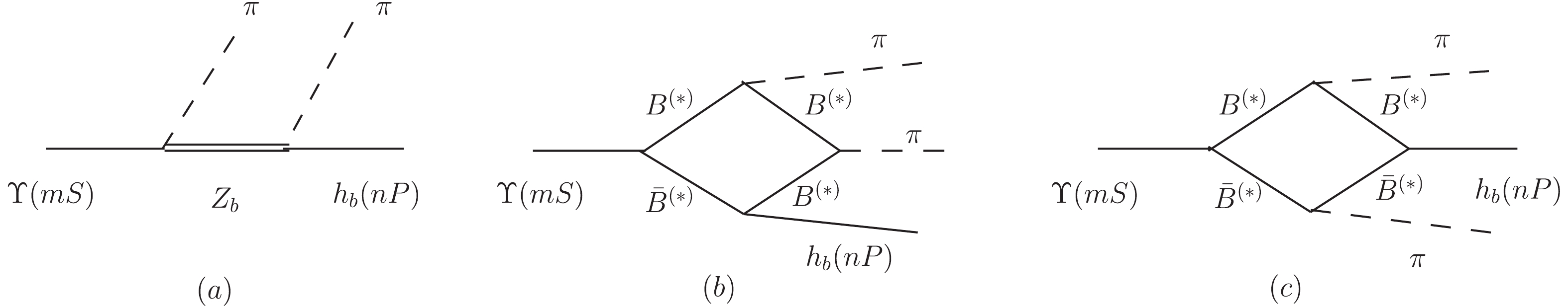
Figure 1. Feynman diagrams considered for
Υ(mS)→hb(nP)ππ processes. Crossed diagrams of (a) and (b) are not shown explicitly.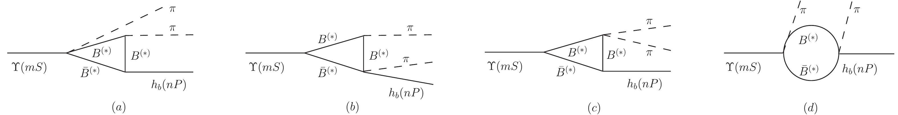
Figure 2. Loop diagrams not considered in the calculations. The corresponding power counting arguments are given in the main text.
First, we analyze the power counting of the box diagrams, namely Fig. 1(b), (c). As shown in Eq. (7), the vertex of
B(∗)B(∗)π is proportional to the external momentum of the pionqπ . TheΥB(∗)ˉB(∗) vertex is in a P-wave, and thehbB(∗)ˉB(∗) vertex is in an S-wave; therefore, the loop momentum must contract with the external pion momentum, and hence the P-wave vertex scales asO(qπ) . Thus, the box diagrams scales asν5q3π/ν8=q3π/ν3. For the triangle diagram Fig. 2(a), the leading
ΥB(∗)ˉB(∗)π vertex given bygJHHπ⟨JˉH†aH†b⟩u0ab [37] is proportional to the energy of the pion,Eπ∼qπ . Therefore, Fig. 2(a) is counted asmBν5q2π/ν6=mBq2π/ν , where the factormB is introduced to match the dimension with the scaling for the box diagrams.In Fig. 2(b), the leading
hbB(∗)ˉB(∗)π vertex given byghbHHπ⟨h†ibHaσjˉHb⟩ϵijkukab [29] is proportional to the momentum of the pionqπ . The loop momentum due to theΥB(∗)ˉB(∗) coupling has to contract with the external pion momentum. Thus, Fig. 2(b) scales asν5q3π/ν6=q3π/ν .The leading
B(∗)B(∗)ππ vertex comes from the chiral derivative term⟨H†a(iD0)baHb⟩=⟨H†a(i∂0−iV0)baHb⟩ [38, 39], in which the pion pair produced by the vector current,Vμ=12(u†∂μu+u∂μu†) , cannot form a positive-parity and C-parity state; therefore, this leading vertex does not contribute to theΥ(mS)→hb(nP)ππ processes. Isoscalar,PC=++ pion pairs only enter in the next orderO(q2π) from point vertices. Therefore, Fig. 2(c) scales asν5q3π/ν6=q3π/ν .In Fig. 2(d), both the initial and final vertices are proportional to
qπ ; therefore, the bubble loop scales asmBν5q2π/ν4=mBq2πν .Therefore, we expect that the ratios of the contributions of the box diagrams, triangle diagram Fig. 2(a)–(c), and the bubble loop Fig. 2(d) are
q3πν3:mBq2πν:q3πν:q3πν:mBq2πν=1:mBν2qπ:ν2:ν2:mBν4qπ,
(8) where
qπ≃(mΥ(4S)−mhb(nP))/2 andν=(νΥ(4S)+νhb(nP))/2 , withνΥ(4S)≃0.06 ,νhb(1P)≃0.35 , andνhb(2P)≃0.24 . Thus, for theΥ(4S)→hb(1P)π+π− transition, the ratios in Eq. (8) are1:0.67:0.04:0.04:0.03 . For theΥ(4S)→hb(2P) π+π− transition, the ratios are1:0.75:0.02:0.02:0.02 . Therefore, according to the power counting, the box diagrams and triangle diagram in Fig. 2(a) are dominant among the loop contributions, and they are of the same order. TheΥ(4S) is below theB(∗)ˉB(∗)π threshold, and the couplinggJHHπ in the triangle diagram Fig. 2(a) is unknown. Thus, for a rough estimation of the loop contributions, we will only calculate the box diagrams in the present study. All the box and triangle loop contributions discussed here are ultraviolet-finite and do not require additional introduction of counterterms. -
The decay amplitude for
Υ(mS)(pa)→hb(nP)(pb)π(pc)π(pd)
(9) is described in terms of the Mandelstam variables
s=(pc+pd)2,t=(pa−pc)2,u=(pa−pd)2.
(10) By using the effective Lagrangians in Eqs. (1) and (2), the tree amplitude of
Υ(mS)→Zbπ→hb(nP)ππ can be obtained asMZb=2√mΥ(mS)mhb(nP)F2πϵabjϵaΥ(mS)ϵbhb(nP)∑i=1,2mZbiCZbiΥ(mS)πgZbihb(nP)π{p0cpjd1t−m2Zbi+p0dpjc1u−m2Zbi}.
(11) The nonrelativistic normalization factor
√mY has been multiplied with the amplitude for every heavy particle, withY=Υ(mS),hb(nP),Zbi . The widths of theZb states are neglected in the present study, because they are of the order of10MeV and are considerably smaller than the difference between theZb masses and theΥ(mS)π/hb(nP)π threshold.Now, we discuss the calculation of the box diagrams. In the box diagrams Fig. 1(b) and (c), we denote the top left intermediate bottom meson as M1, and the other intermediate bottom mesons as M2, M3, and M4, in counterclockwise order. For the pseudoscalar or vector content of
[M1,M2,M3,M4] , there are twelve possible patterns and we number them in order: 1,[PPPV] ; 2,[PPVV] ; 3,[PVPV] ; 4,[PVVP] ; 5,[VVPP] ; 6,[VPVP] ; 7,[VPPV] ; 8,[PVVV] ; 9,[VPVV] ; 10,[VVPV] ; 11,[VVVP] ; 12,[VVVV] . For each pattern, we also need to consider six possibilities of different flavor of the intermediate bottom mesons:[B(∗)+,B(∗)−,B(∗)+,B(∗)0] ,[B(∗)+,B(∗)−, ˉB(∗)0,B(∗)0] ,[B(∗)0,ˉB(∗)0,B(∗)0,B(∗)+] ,[B(∗)−,B(∗)+,B(∗)−,ˉB(∗)0] ,[ˉB(∗)0,B(∗)0,B(∗)+,B(∗)−] , and[ˉB(∗)0,B(∗)0,ˉB(∗)0,B(∗)−] . The full amplitude contains the sum of all possible amplitudes.For the tensor reduction of the loop integrals, it is convenient to define
q=−pb and thperpendicular momentumq⊥=pc−q(q⋅pc)/q2 , which satisfyq⋅q⊥=0 . The result of the amplitude of the box diagrams can be written asMloop=ϵaΥ(mS)ϵbhb(nP){ϵabiqiA1+ϵabiqi⊥A2+ϵbijqiqj⊥qa⊥A3+ϵbijqiqj⊥qaA4+ϵaijqiqj⊥qb⊥A5+ϵaijqiqj⊥qbA6}.
(12) Details on the analytic calculation of the box diagrams and explicit expressions of
Ai (i=1,2,...,6) are given in Appendix A.The decay width for
Υ(mS)→hb(nP)ππ is given byΓ=∫s+s−∫t+t−|MZb+Mloop|2dsdt768π3m3Υ(mS),
(13) where the lower and upper limits are given as
s−=4m2π,s+=(mΥ(mS)−mhb(nP))2,t±=14s{(m2Υ(mS)−m2hb(nP))2−[λ12(s,m2π,m2π)∓λ12(m2Υ(mS),s,m2hb(nP))]2},λ(a,b,c)=a2+b2+c2−2(ab+ac+bc).
(14) -
To estimate the contribution of the
Zb -exchange mechanism, we need to know the coupling strengths ofZbΥ(4S)π andZbhb(nP)π . The mass difference betweenZb(10610) andZb(10650) is considerably smaller than the difference between their masses and theΥ(mS)π/hb(nP)π threshold, and they have the same quantum numbers, and thus the same coupling structures as given by Eqs. (1) and (2). Therefore, it is very difficult to distinguish their effects from each other in the dipion transitions ofΥ(4S) , so we only used oneZb , theZb(10610) , which approximately combines bothZb states' effects. In Ref. [26], we studied theΥ(4S)→Υ(mS)ππ processes to extract the coupling constant|CZbΥ(4S)π|=(3.3±0.1)×10−3 , which combine the effects from bothZb states. For the couplings ofZbhb(nP)π , in principle, they can be extracted from the partial widths of theZb states decay intohb(nP)π(n=1,2) |gZbhbπ|={6πF2πmZbΓZb→hbπ|pf|3mhb}12,
(15) where
|pf|≡λ1/2(m2Zb,m2hb,m2π)/(2mZb) . The branching fractions of the decays of bothZb states intohb(nP)π(n=1,2) has been given in [40], where theZb line shapes were described using Breit-Wigner forms. If we naively use these branching fractions, we would obtain|gnaiveZb1hb(1P)π|=0.019±0.003,|gnaiveZb2hb(1P)π|=0.021±0.003,|gnaiveZb1hb(2P)π|=0.068±0.011,|gnaiveZb2hb(2P)π|=0.077±0.010.
(16) Here, all the
Zbhbπ couplings are labeled by a superscript "naive" because this is not the appropriate way to extract coupling strengths in this case; theZb states are very close to theB(∗)ˉB∗ thresholds. Therefore, the Flatté parametrization for theZb spectral functions should be used, which will lead to much larger partial widths into(bˉbπ) channels, and thus the relevant coupling strengths. As analyzed in Ref. [41], in the the Flatté parametrization the sum of the partial widths of theZb(10610) other than that for theBˉB∗ channel should be greater than the nominal width, which is approximately20MeV . While summing over all theΥ(nS)π(n=1,2,3) andhb(mP)π(m=1,2) , and the branching fractions in Ref. [40] is approximately 14% or3MeV in terms of partial widths. Therefore, for a rough estimation, we use three times the results of Eq. (16):|gZbhb(1P)π|≃0.057,|gZbhb(2P)π|≃0.204.
(17) We find that even after considering the enlarging factor of three for the couplings
|gZbhb(nP)π| , theZb -exchange contribution is still considerably smaller than the bottom meson loops contributions.In the calculation of the box diagrams, the coupling strength
gJHH(4S) can be extracted from the measured open-bottom decay widths of theΥ(4S) , and we havegJHH(4S)=1.43±0.01GeV−3/2 . For thehbB∗ˉB∗ couplingg1 , we can use the results from Ref. [27]. In [27], theZb -exchange mechanism in theΥ(5S)→hb(1P,2P)ππ processes was studied assuming theZb states areB(∗)ˉB∗ bound states and the physical coupling of theZb states to the bottom and anti-bottom mesons,z1 , as well as the productg1z1 was determined. By using their resultsz1=0.75+0.08−0.11GeV−1/2 andg1z1=0.40±0.06GeV−1 , we can extract thatg1=0.53+0.19−0.13GeV−1/2 . In [27], in order to reduce the number of free parameters, the couplings ofhb(1P)B∗ˉB∗ andhb(2P)B∗ˉB∗ are assumed to be the same.By using the coupling strengths above, we can predict the decay branching fractions of
Υ(4S)→ hb(1P,2P)π+π− . Depending on the sign of the couplings in Eq. (17), the interferences can be constructive or destructive between theZb -exchange and box graph mechanisms; therefore, there are two possible results for each processBRΥ(4S)→hb(1P)π+π−≃(1.2+0.8−0.4×10⁻⁶)or(0.5+0.5−0.2×10⁻⁶),BRΥ(4S)→hb(2P)π+π−≃(7.1+1.7−1.1×10⁻¹⁰)or(2.4+0.2−0.1×10⁻¹⁰).
(18) We find that the
BRΥ(4S)→hb(1P)π+π− is at least one order of magnitude smaller than the branching fractionsBRΥ(4S)→Υ(1S,2S)π+π− , which are approximately8×10−5 given in PDG [42], and theBRΥ(4S)→hb(2P)π+π− is small owing to the very small phase space. We discuss theΥ(4S)→hb(1P)π+π− transition in further detail. To illustrate the effects of theZb -exchange and box graph mechanisms inΥ(4S)→ hb(1P)ππ , we give the predictions only including theZb -exchange terms or only including the box diagramsBRZbΥ(4S)→hb(1P)π+π−=0.6+0.1−0.1×10⁻⁷,BRBoxΥ(4S)→hb(1P)π+π−=0.8+0.7−0.3×10⁻⁶.
(19) We can observe that the bottom meson loops contribution is considerably larger than the
Zb -exchange contribution, while it is two orders of magnitude smaller than theΥ(4S)→ Υ(1S,2S)π+π− transitions. Note that the direct gluon hadronization mechanism contribution within QCDME for theΥ(4S)→hb(1P)π+π− process has not been calculated thus far. In references [5–8], QCDME predict that the branching fraction ofΥ(3S)→hb(1P)ππ is 2-3 orders of magnitude suppressed compared to ofΥ(3S)→Υ(1S)ππ . The three orders of magnitude suppression is supported by experiment [9]. Because the mass difference between theΥ(4S) andhb(1P) is approximately 0.68 GeV, the pions in theΥ(4S)→hb(1P)π+π− process can also be considered to be in the soft region. If one approximates that the gluon hadronization mechanism within QCDME inΥ(4S)→hb(1P)π+π− is also 2-3 orders of magnitudes suppressed compared to that in theΥ(4S)→Υ(1S)π+π− process, as in theΥ(3S) decay cases. Then, the gluon hadronization mechanism contribution is at most at the same order of the bottom meson loops contribution. Owing to the lack of exact information on the gluon hadronization within QCDME and the neglecting of the triangle diagram Fig. 2(a) as discussed in section 2.3, it is important to note that the results presented in this paper are order-of-magnitude estimates.In Fig. 3, we plot the distributions of the
ππ andhbπ invariant mass spectra, and the distribution of cosθ , whereθ is defined as the angle between the initialΥ(mS) and theπ+ in the rest frame of theππ system. To illustrate the effects of different mechanisms, the contributions of the box diagrams,Zb -exchange, their sum with the constructive interference, and the sum with destructive interference are indicated by dark green dashed, magenta dotted, red solid, and blue dot-dashed lines, respectively. There is a broad bump at approximately 0.5 GeV in the dipion invariant mass distribution. Theππ invariant mass spectra with unknown normalization predicted within QCDME in Ref. [5] showed a peak at lowππ masses. Thus, theππ invariant mass spectra can be useful to identify the effects of the bottom meson loops and the gluon hadronization mechanism with future experimental data. Further, the angular distribution is far from flat. In theΥ(mS)→ hb(nP)ππ process, the isospin conservation combined with Bose symmetry requires the pions to have even relative angular momentum. Therefore, there is a large D-wave component from the box diagrams if higher partial waves are neglected.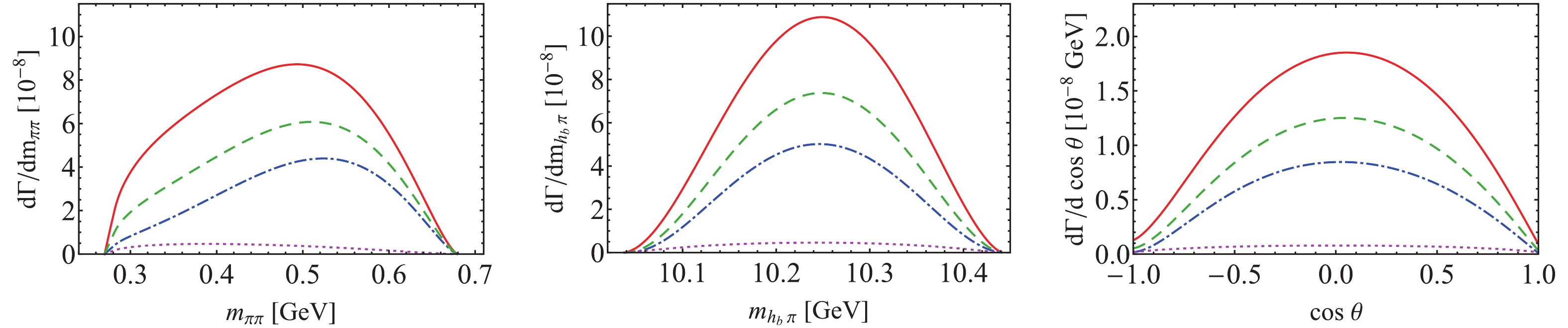
Figure 3. (color online) Theoretical predictions of the distributions of the
ππ andhbπ invariant mass spectra, and helicity angular distributions in theΥ(4S)→hb(1P)ππ process. Dark green dashed, magenta dotted, red solid, and blue dot-dashed lines represent the contributions of the box diagrams,Zb -exchange, their sum with constructive interference, and the sum with destructive interference, respectively.The
Υ(mS)→hb(nP)ππ are heavy quark spin flip processes, and they are forbidden in the heavy quark limit. We checked that in the heavy quark limit, i.e.mB=mB∗ , all the box diagrams were cancelled with each other; therefore, the bottomed loops did not contribute to theΥ(mS)→hb(nP)ππ transitions. With the small mass splitting of B andB∗ in the real world, as shown in Eqs. (18) and (19), the bottomed meson loops contribution does not produceΥ(4S)→hb(1P)ππ at a rate comparable to the heavy quark spin conservedΥ(4S)→Υ(1S,2S)ππ transitions. Note that the datasets collected atΥ(4S) by BABAR and Belle II collaborations are471×106 and772×106 [43], respectively. Thus, they should contain several hundreds ofΥ(4S)→hb(1P)ππ events according to our calculation. We hope future experimental analysis by BABAR and Belle can test our predictions. As stated in the introduction, the observedΥ(5S)→hb(nP)π+π− proceed at a rate comparable to theΥ(5S)→Υ(lS)π+π− processes [10, 11]. The enhancements may be caused by the effects of the on-shellZb exchange and the two-cut condition complexity of the bottom meson loops in theΥ(5S) decays. A detailed analysis of theΥ(5S)→ hb(nP)π+π− processes is beyond the scope of this study.Owing to the similarity between the bottomonium and charmonium families, we can extend the box diagrams calculation to give a rough estimation of the branch fractions of the
ψ(3S)(ψ(4040))→hc(1P)π+π− andψ(4S) (ψ(4415))→hc(1P)π+π− transitions. The relevant Feynman diagrams can be obtained by replacing the externalΥ(mS) andhb(nP) byψ(mS) andhc(nP) , respectively, and replacing the intermediateB(∗) byD(∗) in Fig. 1(b) and (c). The experimental decay widths of theψ(3S,4S)→D(∗)ˉD(∗) transitions are not given in PDG, and we will use the theoretical predictions of the decay widths in Ref. [44] to estimate the coupling strengthsgJHH(ψ(3S)) andgJHH(ψ(4S)) . Because among the different decay modesD(∗)ˉD(∗) , theDˉD∗ andD∗ˉD∗ modes are dominant forψ(3S) andψ(4S) , respectively, we will use the corresponding coupling constants in the calculation, namelygJHH(ψ(3S))=gψ(3S)DˉD∗=0.97GeV−3/2 andgJHH(ψ(4S))= gψ(4S)D∗ˉD∗=0.25GeV−3/2 . For thehcD∗ˉD∗ coupling, we use the result from Ref. [45],ghcD∗ˉD∗=−(√mχc0/3)/(fχc0)= −(√3.415/3)/(0.297)GeV−1/2=−3.59GeV−1/2 . The predictions of the box diagrams contributions to the branch fractions ofψ(3S,4S)→hc(1P)π+π− areBRBoxψ(3S)→hc(1P)π+π−=2.9×10⁻⁵,BRBoxψ(4S)→hc(1P)π+π−=4.5×10⁻³.
(20) The prediction of
BRBoxψ(3S)→hc(1P)π+π− is below the upper limit given in PDG [42]. As expected the branch fractionsBRBoxψ(3S,4S)→hc(1P)π+π− are considerably larger thanBRBoxΥ(4S)→hb(1P)π+π− , because the mass splitting of D andD∗ is considerably larger than that of B andB∗ . Note that this is just a preliminary rough estimation, owing to the lack of sufficient information concerning theψ(3S,4S)D(∗)ˉD(∗) coupling constants and the neglecting of the loop diagrams with intermediateD1 state in the present calculation. A detailed theoretical study of theψ(3S,4S)→ hc(1P)π+π− transitions will be pursued in the future. -
In this study, we investigate the effects of
Zb exchange and bottom meson loops in the heavy quark spin flip transitionsΥ(4S)→hb(nP)ππ(n=1,2) . The bottom meson loops are treated in the NREFT scheme, in which the dominant box diagrams are considered. We find that the bottom meson loops contribution is considerably larger than theZb -exchange contribution in theΥ(4S)→ hb(1P)ππ transition, while it can not produce decay rates comparable to the heavy quark spin conservedΥ(4S)→Υ(1S,2S)ππ processes. The theoretical prediction of the decay rate and the dipion invariant mass spectra ofΥ(4S)→hb(1P)ππ in this work may be useful for identifying the effect of the bottom meson loops with future experimental analysis. We also predict the branch fractions ofψ(3S,4S)→hc(1P)ππ contributed from the charm meson loops. -
In this appendix, first, we discuss the parametrization and simplification of the scalar four-point integrals in the box diagrams. Then, we introduce a tensor reduction scheme to deal with higher-rank loop integrals. Finally, we give the amplitude of the box diagrams for the
Υ(mS)→hb(nP)ππ process. -
For the first topology, as shown in Fig. A1, the scalar integral evaluated for the initial bottomonium at rest (
p=(M,0) ) reads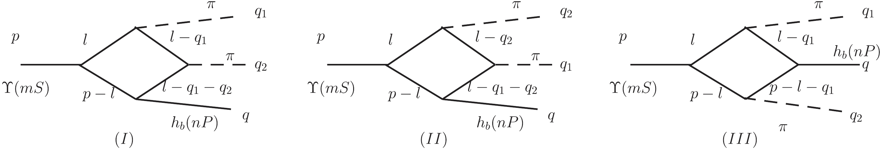
Figure A1. Kinematics used for calculating four-point integrals.
We are grateful to the referees' useful suggestions and constructive remarks, which helped formulate the present version of this manuscript. We are grateful to Martin Cleven for the collaboration in the early stages of this study. We acknowledge Guo-Ying Chen, Meng-Lin Du, and Qian Wang for their helpful discussions, and Feng-Kun Guo for a careful reading of the manuscript and valuable comments.
J(0)1≡i∫d4l(2π)41[l2−m21+iϵ][(p−l)2−m22+iϵ][(l−q1−q2)2−m23+iϵ][(l−q1)2−m24+iϵ]≃−i16m1m2m3m4×∫d4l(2π)41[l0−l22m1−m1+iϵ][l0−M+l22m2+m2−iϵ]1[l0−q01−q02−(l+q)22m3−m3+iϵ][l0−q01−(l−q1)22m4−m4+iϵ].
By performing the contour integration, we find
−μ12μ23μ242m1m2m3m4∫d3l(2π)31[l2+c12−iϵ][l2+2μ23m3l⋅q+c23−iϵ][l2−2μ24m4l⋅q1+c24−iϵ],
where we defined
c12≡2μ12(m1+m2−M),c23≡2μ23(m2+m3−M+q01+q02+q22m3),c24≡2μ24(m2+m4−M+q01+q212m4),μij=mimjmi+mj.
The second topology in Fig. A1 is just the crossed diagram of the first topology with
q1↔q2 , so the scalar integral readsJ(0)2=−μ12μ23μ242m1m2m3m4∫d3l(2π)3×1[l2+c12−iϵ][l2+2μ23m3l⋅q+c23−iϵ][l2−2μ24m4l⋅q2+c′24−iϵ],
where
c′24≡2μ24(m2+m4−M+q02+q222m4).
For the third topology, we have
J(0)3≡i∫d4l(2π)41[l2−m21+iϵ][(p−l)2−m22+iϵ][(p−q2−l)2−m23+iϵ][(l−q1)2−m24+iϵ]≃−i16m1m2m3m4∫d4l(2π)41[l0−l22m1−m1+iϵ][l0−M+l22m2+m2−iϵ]×1[l0+q02−M+(l+q2)22m3+m3−iϵ][l0−q01−(l−q1)22m4−m4+iϵ].
By the contour integration, we find
−μ12μ342m1m2m3m4∫d3l(2π)31[l2+d12−iϵ][l2−2μ34m4l⋅q1−2μ34m3l⋅q2+d34−iϵ]×[μ24[l2−2μ24m4l⋅q1+d24−iϵ]+μ13[l2+2μ13m3l⋅q2+d13−iϵ]],
where we defined
d12≡2μ12(m1+m2−M),d34≡2μ34(m3+m4−q0+q212m4+q222m3),d24≡2μ24(m2+m4−M+q01+q212m4),d13≡2μ13(m1+m3−M+q02+q222m3).
In all the three cases, the remaining three-dimensional momentum integration will be carried out numerically.
-
Because the
ΥB(∗)ˉB(∗) vertex scales with the momentum of the bottom meson pair, for topology I we have to deal with−μ12μ23μ242m1m2m3m4∫d3l(2π)3f(l)[l2+c12−iϵ][l2+2μ23m3l⋅q+c23−iϵ][l2−2μ24m4l⋅q1+c24−iϵ],
where
f(l)={1,li} for the fundamental scalar and vector integrals, respectively. A convenient parametrization of the tensor reduction isJ(1)i1=−μ12μ23μ242m1m2m3m4∫d3l(2π)3li[l2+c1−iϵ][l2−2μ23m3l⋅q+c2−iϵ][l2−2μ24m4l⋅q1+c3−iϵ]≡qiJ(1)1+qi1⊥J(2)1,
where
q1⊥=q1−q(q⋅q1)/q2 . The expressions of the scalar integralsJ(r)1 can easily be disentangled and should be evaluated numerically. The corresponding expressions for topology II and III can be obtained by changing the denominators accordingly. -
We define the scalar integrals
J1(i,r,k) based on theJ(r)1 in the tensor reduction of vector integral in Eq. (A10), wherei=1,2,3 denotes the three topologies of the box diagrams shown in Fig. A1,r=1,2 refers to the two componentsJ(r)1 , andk=1,2,...,12 represents the twelve patterns with different pseudoscalar or vector content of the intermediate bottom mesons in[M1,M2,M3,M4] as displayed in Sec. 2.3.We give the amplitude of the box diagrams for the
Υ(mS)→hb(nP)ππ process, namely theAl(l=1,2,...,6) in the Eq. (12).A1=8g1gJHHg2πF2πq2{q2{pc⋅pd[J1(1,1,3)+J1(2,1,3)+J1(3,1,8)]+pc⋅q[J1(1,1,9)+J1(1,1,11)−J1(2,1,12)+J1(3,1,9)+J1(3,1,11)]+q2⊥[J1(1,2,9)+J1(1,2,11)−J1(2,2,12)+J1(3,2,9)+J1(3,2,11)]}+pc⋅q{pc⋅q[J1(1,1,9)+J1(1,1,11)−J1(2,1,12)+J1(3,1,9)+J1(3,1,11)]+pd⋅q[J1(1,1,12)−J1(2,1,9)−J1(2,1,11)+J1(3,1,10)]+q2⊥[J1(1,2,9)+J1(1,2,11)−J1(1,2,12)+J1(2,2,9)+J1(2,2,11)−J1(2,2,12)+J1(3,2,9)−J1(3,2,10)+J1(3,2,11)]}},
A2=8g1gJHHg2πF2π{pc⋅pd[J1(1,2,3)+J1(2,2,3)+J1(3,2,8)]+pc⋅q[J1(1,1,9)+J1(1,1,11)−J1(2,1,12)+J1(3,1,9)+J1(3,1,11)]+pd⋅q[J1(1,1,12)−J1(2,1,9)−J1(2,1,11)+J1(3,1,10)]+q2⊥[J1(1,2,9)+J1(1,2,11)−J1(1,2,12)+J1(2,2,9)+J1(2,2,11)−J1(2,2,12)+J1(3,2,9)−J1(3,2,10)+J1(3,2,11)]},
A3=−8g1gJHHg2πF2πq2{q2[−J1(1,1,9)+J1(1,1,11)−J1(1,1,12)−J1(1,2,2)+J1(1,2,9)+J1(1,2,10)+J1(1,2,12)−J1(2,1,9)+J1(2,1,11)−J1(2,1,12)+J1(2,2,2)−J1(2,2,10)−J1(2,2,11)−J1(3,1,9)−J1(3,1,10)+J1(3,1,11)−J1(3,2,2)+J1(3,2,9)+J1(3,2,10)+J1(3,2,12)]+pc⋅q[J1(1,2,9)−J1(1,2,11)+J1(1,2,12)+J1(2,2,9)−J1(2,2,11)+J1(2,2,12)+J1(3,2,9)+J1(3,2,10)−J1(3,2,11)]},
A4=8g1gJHHg2πF2πq4{q4[J1(1,1,2)−J1(1,1,10)−J1(1,1,11)−J1(2,1,2)+J1(2,1,9)+J1(2,1,10)+J1(2,1,12)+J1(3,1,2)−J1(3,1,11)−J1(3,1,12)]+q2pc⋅q[J1(1,1,9)−J1(1,1,11)+J1(1,1,12)−J1(1,2,9)+J1(1,2,11)−J1(1,2,12)+J1(2,1,9)−J1(2,1,11)+J1(2,1,12)−J1(2,2,9)+J1(2,2,11)−J1(2,2,12)+J1(3,1,9)+J1(3,1,10)−J1(3,1,11)−J1(3,2,9)−J1(3,2,10)+J1(3,2,11))−(pc⋅q)2[J1(1,2,9)−J1(1,2,11)+J1(1,2,12)+J1(2,2,9)−J1(2,2,11)+J1(2,2,12)+J1(3,2,9)+J1(3,2,10)−J1(3,2,11)]},
A5=8g1gJHHg2πF2πq2{q2[−J1(1,1,6)+J1(1,2,8)+J1(1,2,10)−J1(2,1,6)+J1(2,2,6)−J1(2,2,8)−J1(2,2,10)−J1(3,1,3)+J1(3,1,6)−J1(3,1,8)+J1(3,2,3)+J1(3,2,12)]+pc⋅q[J1(1,2,6)+J1(2,2,6)+J1(3,2,3)−J1(3,2,6)+J1(3,2,8)]},
A6=−8g1gJHHg2πF2πq4{q4[J1(1,1,6)−J1(1,1,8)−J1(1,1,10)+J1(2,1,8)+J1(2,1,10)−J1(3,1,6)+J1(3,1,8)−J1(3,1,12)]+q2pc⋅q[J1(1,1,6)−J1(1,2,6)+J1(2,1,6)−J1(2,2,6)+J1(3,1,3)−J1(3,1,6)+J1(3,1,8)−J1(3,2,3)+J1(3,2,6)−J1(3,2,8)]−(pc⋅q)2[J1(1,2,6)+J1(2,2,6)+J1(3,2,3)−J1(3,2,6)+J1(3,2,8)]}.
Figure 1.
Feynman diagrams considered for Υ(mS)→hb(nP)ππ![]()
![]()
processes. Crossed diagrams of (a) and (b) are not shown explicitly.


 DownLoad: