


 Abstract
 HTML
HTML Reference
 Related
 PDF
PDF


-
A black hole (BH) is a physical object that has the ability to absorb all types of energy from its surroundings as a result of its strong gravitational pull. According to the theory of general relativity, a BH attracts all types of particles that interact with the event horizon. Hawking (1974) described that a BH acts as a black body and emits particles in the form of radiation through its horizon Considering quantum effects in the background of curved spacetime, this radiation is known as Hawking radiation [1] and exhibits a particular temperature, called the Hawking temperature. Quantum tunneling proved to be one of the best techniques [2-4] employed to study the Hawking radiation phenomenon. This technique depends on electron-positron pair-creation, which requires an electric field. As particles overcome the horizon, their energy changes the sign, such that a member of the pair created just inside/outside the horizon can materialize with zero total energy, while the other has the ability to tunnel to the opposite side of the horizon [5].
According to the tunneling phenomenon, particles are permitted to follow classically forbidden trajectories, by starting from outside the horizon to infinity [6, 7]. BH evaporation can be studied with the discharge of quantum particles in form of Hawking radiation, which enables a BH to lose its mass. When a BH loses more matter than it gains through different means it disseminates, shrinks, and eventually disappears. This phenomenon causes a change in the thermodynamical characteristic of a BH, i.e., charge, mass, and angular momentum. These particles follow the frame of outgoing/ingoing radial null geodesics. For outgoing geodesics, the particles must be imaginary, although for ingoing geodesics, they are considered to be real. This is because only a real particle that has a speed, which is not exactly or equivalent to the speed of light can exist inside the horizon.
To calculate the imaginary part of the classical action, there are two main approaches, i.e., null geodesic technique and Hamilton-Jacobi strategy. The first one proposed by Parikh and his colleagues [5] and second one introduced by Srinivasan and Padmanabhan [6]. To construct a relation between classical and quantum theory, an approximation is known as WKB approximation utilized by Wentzel, Kramers, and Brillouin (WKB) [8]. Various authors studied the tunneling of vector particles, bosonic particles, spin-2, spin-3/2, and fermionic particles to obtain the Hawking temperature for different BHs and wormholes [9-59].
By incorporating generalized uncertainty principle (GUP) effects, it is conceivable to discuss quantum-corrected thermodynamical properties of BH [60]. The GUP provides high-energy remedies to BH thermodynamics, which leads to the possibility of a minimal length in quantum gravity theory. According to the modified fundamental commutation relation
$[x_i, p_i] = i\hbar\delta_{ij} $ $ [1+\beta p^2]\; $ [61, 62], the GUP expression can be given as$ {\Delta x\Delta p \geqslant \frac{\hbar}{2}\left[1+\beta(\Delta p)^2\right],} $

(1) where
$ \beta = \frac{\beta_0}{M_p^2} $ ,$ \beta_0 $ denotes the dimensionless parameter, and$ \beta_0<10^{5} $ , the$ {M_p^2} $ depicts the Plank mass. The$ x_i $ and$ p_i $ stand for modified position and momentum operators, respectively. They can be defined as$ x_i \!\!=\!\! x_{0i}, p_i \!\!=\!$ $ p_{0i}\left(1+\beta p^2_{0i}\right), $ where$ x_{0i} $ and$ p_{0i} $ are standard position and momentum operators, respectively, which satisfy the usually commutation relation$ [x_{0i}, p_{0i}] = i\hbar\delta_{ij} $ . We have considered the values of$ \beta $ according to this condition, which also satisfies the condition of GUP relation [63]. For corrections of the Hawking temperature, we have considered only the first order terms of$ \beta $ in our calculation. The idea of GUP has been utilized for various BHs. The tunneling process for Kerr, Kerr-Newman, and Reissner-Nordström (RN) BHs [64] provides an important contribution towards the BH physics. Jiang [65] calculated the tunneling of Dirac particles and analyzed the Hawking radiation spectrum for a black ring. Jian and Bing-Bing [66] studied the fermion particles tunneling from uncharged and charged BHs. Yale [67] studied the scalar, fermion, and boson particles tunneling from BHs without back-reaction effects, they also analyzed the exact Hawking temperature for these particles. Sharif and Javed [68] studied the Hawking radiation through the quantum tunneling process for various types of BHs and also derived the tunneling probabilities as well as their corresponding Hawking temperatures. The same authors [69] calculated the tunneling behavior of fermion particles from traversable wormholes. They also discussed the tunneling behavior of fermion particles for charged accelerating rotating BHs associated with the NUT parameter [70].$ \ddot{\rm{O}} $ vg$ \ddot{\rm{u}} $ n et al. [71] calculated the tunneling rate of charged massive bosons for various types of BHs surrounded by the perfect fluid in Rastall theory. Anacleto et al. [72] studied the finite quantum-corrected entropy from non-commutative acoustic BHs. Li and Zu [73] analyzed GUP effects by applying the Klein-Gordon equation and also studied corrected temperature for Gibbon-Maeda-Dilation BH. Anacleto et al. [74] investigated the quantum-corrected entropy using a tunneling method with GUP in self-dual BH. Övgün and Jusufi [75] studied spin-$ 1 $ vector particles tunneling for charged non-commutative BHs and their GUP-corrected thermodynamical properties. Singh et al. [76] analyzed the particle radiation for Kerr-Newman BH using the quantum tunneling phenomenon. Sakalli et al. [77] investigated the scalar particles tunneling from acoustic BHs with a rotation parameter by applying the WKB approximation and Klein-Gordon equation with GUP to obtain the Hawking temperature of massive particles.Javed et al. [78] analyzed the charged vector particles tunneling phenomenon for a pair of accelerating and rotating, as well as 5D gauged super-gravity BHs and investigated the corresponding Hawking temperatures. As a continuation of their work, we study the Hawking radiation phenomenon by considering quantum corrections of boson particles through the event horizon of accelerating and rotating BH with the NUT parameter. We also discuss the graphical behavior of the corrected temperature with respect to the horizon for a given BH and analyzed the effects of different parameters on temperature and visualize the stable and unstable states of the BH. The main motivation of this work is to study the charged accelerating and rotating black hole with NUT parameters under the influence of quantum gravity, and to investigate how the results reduce to the previously obtained results when we neglect quantum gravity effects and other parameters. The organization of this study is as follows: In section 2, we study the quantum-corrected tunneling rate and correct the Hawking temperature for charged BH solution with acceleration, rotation, and NUT parameter. Moreover, we analyze the graphical behavior of corrected temperature with respect to the event horizon of BH and discuss the effects of different parameters on the temperature. Section 3 is based on the conclusion and discussion of the mathematical results for these BHs.
-
Universally, the NUT parameter is associated with the twisting behavior of the surrounding spacetime or with the gravito-magnetic monopole parameter of the central mass. The precise physical significance of the NUT parameter might not be investigated. In contrast, the higher dimensional origin of the Kerr-NUT-(anti) de-Sitter BH and its physical significance was studied [79, 80]. For a BH, the apparent dominance of the NUT parameter on the rotation parameter removes the metric free of curvature singularity, and the corresponding result is known as the NUT-like result. When the rotation parameter commands the NUT parameter, the solution is Kerr-like, and a ring curvature singularity occurs. This type of singularity is independent from the existence of the cosmological constant.
The exact understanding of the NUT parameter is conceivable when a static Schwarzschild mass is submerged in a stationary source-free electromagnetic universe [81]. Moreover, the NUT parameter is associated with the representation of twisting behavior of the electromagnetic universe, allowing off-Schwarzschild central mass. When electric and magnetic fields vanish, the NUT parameter represents the twist of the vacuum spacetime [70]. Consequently, for the creation of the NUT parameter, the bending of the environmental space couples with the mass of the background field.
The line-element of this BH can be defined as follows [82]
$ \begin{split} {\rm d}s^{2} =& -\frac{1}{\Omega^{2}}\Big[-\frac{Q}{\rho^{2}}\Big( (4l\sin^{2}\frac{\theta}{2}+a\sin^{2}\theta){\rm d}\phi-{\rm d}t\Big)^{2} -\frac{\rho^{2}}{Q}{\rm d}r^{2}\\ &+\frac{\tilde{P}}{\rho^{2}} \Big(((l+a)^{2}+r^{2}){\rm d}\phi-a {\rm d}t\Big)^{2} -\sin^{2}\theta\frac{\rho^{2}}{\tilde{P}} {\rm d}\theta^{2}\Big], \end{split} $

(2) where
$ \begin{array}{l} \Omega = -(a\cos\theta+l)\frac{\alpha}{\omega}r+1 ,\; \; \; \rho^{2} = (a\cos\theta+l)^{2}+r^{2}, \end{array} $

(3) $ \begin{split} Q =& \left[(\tilde{e}^{2}+\omega^{2}\tilde{k}+\tilde{g}^{2})(1+2l\alpha \frac{r}{\omega})-2rM-\displaystyle\frac{\omega^{2}\tilde{k}r^{2}}{l^{2}-a^{2}}\right]\\ &\times \left[1-\frac{l-a}{\omega}\alpha r\right]\left[1-\displaystyle\frac{l+a}{\omega}r\alpha\right] , \end{split} $

(4) $ \begin{array}{l} \tilde{P} = -\sin^{2}\theta(a_{4}\cos^{2}\theta+a_{3}\cos\theta-1) = \sin^{2}\theta P, \end{array} $

(5) $ \begin{array}{l} a_{3} =\displaystyle \frac{\alpha a}{\omega}2M-4\displaystyle\frac{\alpha^{2}al}{\omega^{2}} (\tilde{g}^{2}+\tilde{e}^{2}+\omega^{2}\tilde{k}), \end{array} $

(6) $ \begin{array}{l} a_{4} = -\displaystyle\frac{\alpha^{2}a^{2}}{\omega^{2}}(\tilde{g}^{2}+\tilde{e}^{2}+\omega^{2}\tilde{k}) , \end{array} $

(7) where
$ M $ ,$ g $ , and$ e $ represent mass, magnetic charge, and electric charge, respectively;$ l $ ,$ \omega $ , and$ \alpha $ are the NUT parameter, rotation, and acceleration of source, respectively. Moreover,$ a $ is rotation parameter (parameter of Kerr-like), and$ \tilde{k} $ is defined as$ \left(\frac{\omega^{2}}{l^{2}-a^{2}}-3\alpha^{2}l^{2}\right) \tilde{k} = 3\frac{\alpha^{2}l^{2}}{\omega^{2}}(\tilde{e}^{2}+\tilde{g}^{2}) -2\frac{\alpha l} {\omega}M-1. $

(8) We observe that
$ \omega $ depends on$ a $ and$ l $ . The parameter$ \alpha $ represents the bending behavior of BHs relative to the rotation parameter ($ \omega $ ). The parameters$ \tilde{e} $ ,$ \tilde{g} $ ,$ M $ ,$ \omega $ ,$ \tilde{k} $ , and$ \alpha $ are independent. As$ \alpha = 0 $ , the line-element (2) implies the Kerr-Newman NUT results. For$ l = 0 $ , the line-element (2) yields the BHs with rotating and charged parameters. When$ \tilde{g} $ and$ \tilde{e} $ approach zero, we obtain a Schwarzschild BH, and if$ a $ and$ l $ approach zero, the C-metric is implied.The line-element (2) can be rewritten in the following form
$\begin{split} {\rm d}{s^2} = & - Z(r,\theta ){\rm d}{t^2} + \frac{{{\rm d}{r^2}}}{{B(r,\theta )}} + C(r,\theta ){\rm d}{\theta ^2} \hfill \\ & + D(r,\theta ){\rm d}{\phi ^2} - 2F(r,\theta ){\rm d}\phi {\rm d}t, \hfill \\ \end{split} $

(9) where the metric functions Z, B, C, D, and F are given as follows
$ \begin{array}{l} Z(r, \theta) = \displaystyle\frac{-Pa^2\sin^2\theta+Q}{\Omega^2\rho^2},\;\;\; B(r, \theta) =\displaystyle \frac{\Omega^2 Q}{\rho^2},\;\; C(r, \theta) = \displaystyle\frac{\rho^2}{P\Omega^2}, \end{array} $

(10) $ \begin{array}{l} D(r, \theta) \!= \!\!\displaystyle\frac{1}{\rho^2\Omega^2}\Big({\rm sin}^2\theta Q((a\!+\!l)^2\!+\!r^2)^2\!-\!Q(4l\sin^2\frac{\theta}{2}\!+\!a\sin^2\theta)^2\Big), \end{array} $

(11) $ \begin{array}{l} F(r, \theta) \!=\! \displaystyle\frac{1}{\rho^2\Omega^2}\Big(Pa {\rm sin}^2\theta ((l\!+\!a)^2\!+\!r^2)-Q(4l\sin^2\frac{\theta}{2}\!+\!a\sin^2\theta)\Big). \end{array} $

(12) The electromagnetic potential for this pair of BHs is defined as
$ \begin{split} A =& \displaystyle\frac{1}{a((a{\rm cos}\theta+l)^2+r^2)}\Big[\tilde{g}\Big(-l-a\cos\theta\Big(a {\rm d}t-\Big(r^2+(a+l)^2\Big){\rm d}\phi\\ & + r\tilde{e}\Big({\rm d}\phi((a+l)-a{\rm d}t +(2al\cos\theta+a^2\cos^2\theta+l^2))\Big) \Big]. \end{split} $

(13) The horizons are obtained from
$ B(r, \theta) = \frac{\Omega^2 Q}{\rho^2} = 0 $ , which implies that$ \Omega $ is not zero, thus$ Q $ is zero, such that r has real roots, i.e.,$\begin{split} {r_{\alpha 1}} =& \frac{\omega }{{\alpha (l + a)}},\quad {r_{\alpha 2}} = - \frac{\omega }{{(a - l)\alpha }},\quad \hfill \\ {r_ \pm } = &\frac{{{l^2} - {a^2}}}{{{\omega ^2}\tilde k}}\bigg[(({{\tilde g}^2} + {{\tilde e}^2} + {\omega ^2}\tilde k)\frac{{\alpha l}}{\omega } - M) \hfill \\ \\ & { \pm \sqrt {{{(({{\tilde g}^2} + {{\tilde e}^2} + {\omega ^2}\tilde k)\frac{{\alpha l}}{\omega } - M)}^2} + ({{\tilde g}^2} + {{\tilde e}^2} + {\omega ^2}\tilde k)\frac{{{\omega ^2}\tilde k}}{{{l^2} - {\alpha ^2}}}} \bigg].} \end{split}$

(14) Here,
$ r_{\alpha1} $ and$ r_{\alpha2} $ represent the acceleration horizons, and$ r_\pm $ denotes the inner and outer horizons, such that$ {\Big((\tilde{g}^2+\tilde{e}^2+\omega^2\tilde{k})\frac{\alpha l}{\omega}-M\Big)^2-(\tilde{g}^2+\tilde{e}^2+\omega^2\tilde{k})\frac{\omega^2\tilde{k}}{a^2 -l^2}}>0. $

(15) The angular velocity of BH at outer horizon is given as follows
$ {{\Omega}_H} = \frac{a}{(a+l)^2+r^2_+}. $

(16) To study the corrected tunneling rate for vector bosons through the pair of BHs horizon, we consider the Lagrangian equation with quantum gravity effects. Considering a spacetime with a potential due to both the electric and magnetic field, the behavior of massive (spin-1) vector is described by the wave equation. The GUP modified Lagrangian equation with vector field
$ \psi_{\mu} $ for vector bosons can be expressed as [56, 83]$\begin{split} £^{\rm GUP} = & - \frac{1}{2}(\mathfrak{D}_\mu ^ + \psi _\nu ^ + - \mathfrak{D}_\nu ^ + \psi _\mu ^ + )({\mathfrak{D}^{ - \mu }}{\psi ^{ - \nu }} - {\mathfrak{D}^{ - \nu }}{\psi ^{ - \mu }}) \hfill \\ & - \frac{\iota }{\hbar }e{F^{\nu \mu }}\psi _\mu ^ + \psi _\nu ^ - + \frac{{{m^2}}}{{{\hbar ^2}}}\psi _\mu ^ + {\psi ^{ - \nu }}. \hfill \\ \end{split} $

(17) The modified wave equation for massive vector bosons can be defined as follows
$\begin{split} {{\partial _\mu }}&{(\sqrt { - g} {\psi ^{\nu \mu }}) + \sqrt { - g} \frac{{{m^2}}}{{{\hbar ^2}}}{\psi ^\nu } + \sqrt { - g} \frac{\iota }{\hbar }e{A_\mu }{\psi ^{\nu \mu }} + \sqrt { - g} \frac{\iota }{\hbar }e{F^{\nu \mu }}{\psi _\mu }} \\ & { + \beta {\hbar ^2}{\partial _0}{\partial _0}{\partial _0}(\sqrt { - g} {g^{00}}{\psi ^{0\nu }}) - \beta {\hbar ^2}{\partial _i}{\partial _i}{\partial _i}(\sqrt { - g} {g^{ii}}{\psi ^{i\nu }}) = 0,} \end{split}$

(18) where
$ \mid g\mid $ ,$ m $ , and$ \psi^{\mu\nu} $ are the matrix coefficients, mass of a particle, and anti-symmetric tensor respectively. The anti-symmetric tensor can be defined as$\begin{split} {{\psi _{\nu \mu }}} = &{(1 - \beta {\hbar ^2}\partial _\nu ^2){\partial _\nu }{\psi _\mu } - (1 - \beta {\hbar ^2}\partial _\mu ^2){\partial _\mu }{\psi _\nu }} \\ & { + (1 - \beta {\hbar ^2}\partial _\nu ^2)\frac{\iota }{\hbar }e{A_\nu }{\psi _\mu } - (1 - \beta {\hbar ^2}\partial _\mu ^2)\frac{\iota }{\hbar }e{A_\mu }{\psi _\nu },} \end{split}$

(19) and
$ \begin{gathered} {F_{\mu \nu }} = {\nabla _\mu }{A_\nu } - {\nabla _\nu }{A_\mu },\;{\text{where}}\;{\nabla _{\text{0}}}{\text{ = }}({\text{1 + }}\beta {\hbar ^{\text{2}}}{{{g}}^{{\text{00}}}}\nabla _{\text{0}}^{\text{2}}){\nabla _{\text{0}}}, \hfill \\ {\nabla _{\text{i}}}{\text{ = }}({\text{1 - }}\beta {\hbar ^{\text{2}}}{{{g}}^{{{ii}}}}\nabla _{{i}}^{\text{2}}){\nabla _{{i}}}, \hfill \\ \end{gathered} $

(20) where
$ \beta $ is the representation of the quantum gravity effect in terms of the correction parameter, if$ \beta = 0 $ then the above wave equation reduces to the expressions given in Ref. [78], and if$ A = 0 $ then the above wave equation converts into the expressions given in Ref. [71]. Moreover, if both$ \beta $ and$ A $ are zero, then this wave equation reduces to the wave equation given in Ref. [76]. While$ A_\mu $ is considered as the BH electromagnetic potential,$ e $ denotes the vector bosons charge, and$ \nabla_{\mu} $ represents the covariant derivative. In the equation of wave motion, the$ \psi^{+} $ and$ \psi^{-} $ vector bosons have alike behavior, and the quantum tunneling phenomena for both types of particles is also similar. For the$ +ive $ field, the values of$ \psi^{\mu} $ and$ \psi^{\nu\mu} $ are obtained as follows$ \begin{array}{l} \psi^{0} = \displaystyle\frac{-D\psi_{0}-F\psi_{3}}{ZD+F^{2}},\; \; \; \psi^{1} = B \psi_{1},\\ \psi^{2} = C^{-1} \psi_{2},\; \; \; \psi^{3} = \displaystyle\frac{-F\psi_{0}+Z\psi_{3}}{ZD+F^{2}}, \end{array} $

(21) $ \begin{array}{l} \psi^{01} =\displaystyle \frac{-BD\psi_{01}-BF\psi_{13}}{ZD+F^{2}} ,\; \; \; \psi^{02} = \displaystyle\frac{-D\psi_{02}-F\psi_{23}}{C( ZD+F^{2})}, \\ \psi^{03} =\displaystyle \frac{-\psi_{03}}{ZD+F^{2}}, \end{array} $

(22) $ \begin{array}{l} \psi^{12} \!=\! BC^{-1}\psi_{12},\; \psi^{13} \!=\! \displaystyle\frac{B(Z\psi_{13}-F\psi_{01})}{ZD+F^{2} },\; \psi^{23} \!=\! \displaystyle\frac{B\psi_{23}-F\psi_{02}}{C(ZD+F^{2})}. \end{array} $

(23) Applying the WKB approximation [84]
$ {\psi_{\nu} = c_{\nu}\exp\left[\frac{i}{\hbar}\tilde{I}(t, r, \theta, \phi)\right],} $

(24) where
$ {\tilde{I}(t, r, \theta, \phi) = \tilde{I}_{o}(t, r, \theta,\phi)+{\hbar}\tilde{I}_{1}(t,r,\theta,\phi)+{\hbar}^2\tilde{I}_{2}(t, r, \theta, \phi)}\cdots, $

(25) and (for
$ n = 1, 2,3,4 $ ) in the Lagrangian wave of Eq. (18), ignoring the higher terms, the following set of equations is obtained$ \begin{array}{l} DB[c_{1}(\partial_{0}\tilde{I}_{o})(\partial_{1}\tilde{I}_{o}) -c_{1}\beta(\partial_{0}\tilde{I}_{o})^{3}(\partial_{1}\tilde{I}_{o})+ c_{1}\beta(\partial_{1}\tilde{I}_{o})(\partial_{0}\tilde{I}_{o})^{2} eA_{0} -c_{0}\beta(\partial_{1}\tilde{I}_{o})^{4} +e A_{0}c_{1}(\partial_{1}\tilde{I}_{o})- c_{0}(\partial_{1}\tilde{I}_{o})^{2}]+BF[c_{3}(\partial_{1}\tilde{I}_{o})^{2} \\ + c_{3}\beta(\partial_{1}\tilde{I}_{o})^{3} -c_{1}(\partial_{1} \tilde{I}_{o})(\partial_{3}\tilde{I}_{o})-c_{1}\beta(\partial_{3}\tilde{I}_{o})^{3} (\partial_{1}\tilde{I}_{o}) -eA_{3}c_{1}\beta(\partial_{3}\tilde{I}_{o})^{2} (\partial_{1}\tilde{I}_{o})]+DC^{-1} \times [c_{2}\beta eA_{0}(\partial_{0}\tilde{I}_{o})^{2}(\partial_{2}\tilde{I}_{o}) +c_{2}\beta(\partial_{0}\tilde{I}_{o})^{3}(\partial_{2}\tilde{I}_{o}) \\ - c_{0}\beta(\partial_{2}\tilde{I}_{o})^{2} -c_{0}\beta(\partial_{2}\tilde{I}_{o})^{4} +c_{2}eA_{0}(\partial_{2}\tilde{I}_{o}) +c_{2}(\partial_{0}\tilde{I}_{o}) (\partial_{2}\tilde{I}_{o})]\! +\!F^{-1}[c_{3}(\partial_{2}\tilde{I}_{o})^{2}\! \!+\!c_{3}\beta(\partial_{2}\tilde{I}_{o})^{4} \!-\!c_{2}(\partial_{3}\tilde{I}_{o})(\partial_{2}\tilde{I}_{o})- c_{2}\beta(\partial_{2}\tilde{I}_{o})(\partial_{3}\tilde{I}_{o})^{3}\\ +c_{2}eA_{3}(\partial_{2}\tilde{I}_{o})+c_{2}eA_{3}\beta (\partial_{3}\tilde{I}_{o})^{2} \times (\partial_{2}\tilde{I}_{o})] +[c_{3}(\partial_{3}\tilde{I}_{o}) (\partial_{0}\tilde{I}_{o})-c_{3}\beta(\partial_{0}\tilde{I}_{o})^{3}(\partial_{3}\tilde{I}_{o}) -c_{0}(\partial_{3}\tilde{I}_{o})^{2}-c_{0}\beta(\partial_{3} \tilde{I}_{o})^{4} -c_{0}eA_{3}(\partial_{3}\tilde{I}_{o}) \\ -c_{0}eA_{3}\beta(\partial_{3} \tilde{I}_{o})^{3}+c_{3}eA_{0}(\partial_{3} \tilde{I}_{o}) +c_{3}eA_{0}\beta(\partial_{0}\tilde{I}_{o})^{2} (\partial_{3}\tilde{I}_{o})] +eA_{3}[c_{3}(\partial_{0}\tilde{I}_{o})+c_{3}\beta(\partial_{0}\tilde{I}_{o})^{3}-c_{0}(\partial_{3} \tilde{I}_{o}) +c_{0}\beta(\partial_{3}\tilde{I}_{o})^{3}-c_{3}eA_{0}-c_{3}\beta(\partial_{0}\tilde{I}_{o})^{2} \\ +c_{0}eA_{3}+c_{0}eA_{3} \beta(\partial_{3}\tilde{I}_{o})^{2}] -Dm^{2}c_{0}-Fm^{2}c_{3} = 0, \\ \end{array} $ 
(26) $ \begin{split} & D[c_{1}(\partial_{0}\tilde{I}_{o})^{2} +c_{1}\beta(\partial_{0}\tilde{I}_{o})^{4}- c_{0}(\partial_{0}\tilde{I}_{o})(\partial_{1}\tilde{I}_{o})+c_{0} \beta(\partial_{0}\tilde{I}_{o})(\partial_{1}\tilde{I}_{o})^{3} -e A_{0}c_{1}(\partial_{0}\tilde{I}_{o})+c_{1}\beta(\partial_{0}\tilde{I}_{o})^{3} eA_{0}]+F[c_{3}(\partial_{0}\tilde{I}_{o})(\partial_{1}\tilde{I}_{o})\\ & + c_{3}\beta(\partial_{1}\tilde{I}_{o})^{3}(\partial_{0}\tilde{I}_{o})-c_{1}(\partial_{0} \tilde{I}_{o})(\partial_{3}\tilde{I}_{o}) -c_{1}\beta(\partial_{3}\tilde{I}_{o})^{3} (\partial_{0}\tilde{I}_{o}) -c_{1}eA_{3}(\partial_{0}\tilde{I}_{o}) -eA_{3}c_{1}\beta(\partial_{3}\tilde{I}_{o})^{2} (\partial_{0}\tilde{I}_{o})] +(ZD+F^{2})C^{-1}\\ &\times [ c_{2}(\partial_{1}\tilde{I}_{o})(\partial_{2}\tilde{I}_{o}) +c_{2}\beta(\partial_{1}\tilde{I}_{o})^{3}(\partial_{2}\tilde{I}_{o})- c_{1}\beta(\partial_{2}\tilde{I}_{o})^{2} -c_{1}\beta(\partial_{2}\tilde{I}_{o})^{4}] -m^{2}c_{1}+eA_{0}D[c_{1}(\partial_{0}\tilde{I}_{o}) -c_{1}\beta(\partial_{0}\tilde{I}_{o})^{3} -c_{0}(\partial_{1}\tilde{I}_{o}) \\ & -c_{0}\beta(\partial_{1}\tilde{I}_{o})^{3}+c_{1}eA_{0}+c_{1}eA_{0}\beta (\partial_{0}\tilde{I}_{o})^{2}] +eA_{0}F[c_{3}(\partial_{1}\tilde{I}_{o}) +c_{3}\beta(\partial_{0}\tilde{I}_{o})^{3}\! -\!c_{1}(\partial_{3}\tilde{I}_{o})-c_{0}\beta(\partial_{3} \tilde{I}_{o})^{3}\!-\!c_{1}eA_{3}\!-\!c_{1}eA_{3}\beta(\partial_{3}\tilde{I}_{o})^{2}] \\ & +eA_{0}A[c_{3}(\partial_{1} \tilde{I}_{o})+c_{3}\beta(\partial_{1}\tilde{I}_{o})^{3}-c_{1}(\partial_{3} \tilde{I}_{o})-c_{1}\beta(\partial_{3}\tilde{I}_{o})^{3} -c_{1}eA_{3} -c_{1}\beta(\partial_{3}\tilde{I}_{o})^{2}eA_{3}] +eA_{3}F[c_{1}(\partial_{0} \tilde{I}_{o})+ c_{1}\beta(\partial_{0}\tilde{I}_{o})^{3}-c_{0}(\partial_{1} \tilde{I}_{o})\\ & -c_{0}\beta(\partial_{1}\tilde{I}_{o})^{3}+c_{1}eA_{0}+c_{1}\beta(\partial_{0}\tilde{I}_{o})^{2}eA_{0}] = 0, \end{split} $

(27) $ \begin{array}{l} F[c_{3}(\partial_{0}\tilde{I}_{o})(\partial_{2}\tilde{I}_{o}) +c_{3}\beta(\partial_{0}\tilde{I}_{o})(\partial_{2}\tilde{I}_{o})^{3}- c_{2}(\partial_{0}\tilde{I}_{o})(\partial_{3}\tilde{I}_{o})-c_{2} \beta(\partial_{0}\tilde{I}_{o}) \times (\partial_{3}\tilde{I}_{o})^{3}-eA_{3}c_{2}(\partial_{0}\tilde{I}_{o}) -c_{2}\beta(\partial_{3}\tilde{I}_{o})^{2}(\partial_{0}\tilde{I}_{o}) eA_{0}]+D[c_{2}(\partial_{0}\tilde{I}_{o})^{2}\\ -c_{0}(\partial_{0}\tilde{I}_{o})(\partial_{2}\tilde{I}_{o})+ c_{2}\beta(\partial_{0}\tilde{I}_{o})^{4} \!-\!c_{0}\beta(\partial_{2}\tilde{I}_{o})^{3} (\partial_{0}\tilde{I}_{o})\!+\!c_{2}eA_{0}(\partial_{0}\tilde{I}_{o}) \! +\!eA_{3}c_{2}\beta(\partial_{2}\tilde{I}_{o})^{2}(\partial_{0} \tilde{I}_{o})]\!-\!B[c_{2}(\partial_{1}\tilde{I}_{o})^{2} \!+\!c_{2}\beta(\partial_{1}\tilde{I}_{o})^{4}- c_{1}\beta(\partial_{1}\tilde{I}_{o})(\partial_{2}\tilde{I}_{o})\\ -c_{1}\beta(\partial_{1}\tilde{I}_{o})(\partial_{2}\tilde{I}_{o})^{3}] +B[c_{3}(\partial_{3}\tilde{I}_{o})(\partial_{2}\tilde{I}_{o}) +c_{3}\beta(\partial_{3}\tilde{I}_{o})(\partial_{2}\tilde{I}_{o})^{3}- c_{2}\beta(\partial_{3}\tilde{I}_{o})^{2} -c_{2}\beta(\partial_{3}\tilde{I}_{o})^{4}-eA_{3}c_{2}(\partial_{3}\tilde{I}_{o}) -c_{2}\beta(\partial_{3}\tilde{I}_{o})^{3}eA_{3}] \\ -F[c_{2}(\partial_{0}\tilde{I}_{o})(\partial_{3}\tilde{I}_{o})+c_{2}\beta(\partial_{3}\tilde{I}_{o})(\partial_{0}\tilde{I}_{o})^{3}\!-\! c_{0}\beta(\partial_{2}\tilde{I}_{o})(\partial_{3}\tilde{I}_{o}) \!-\!c_{0}\beta(\partial_{2}\tilde{I}_{o})^{3}(\partial_{3}\tilde{I}_{o})\! +\!e A_{0}c_{2}(\partial_{3}\tilde{I}_{o}) \! +\!c_{2}\beta(\partial_{0} \tilde{I}_{o})^{2}(\partial_{3}\tilde{I}_{o})eA_{0}]-(ZB+F^{2})m^{2}c_{2} \\ +eA_{0}F[c_{3}(\partial_{2}\tilde{I}_{o}) +c_{3}\beta(\partial_{2}\tilde{I}_{o})^{3}-c_{2}(\partial_{3}\tilde{I}_{o}) -c_{2}\beta(\partial_{3}\tilde{I}_{o})^{3}-c_{2}eA_{3}-c_{2}eA_{3}\beta (\partial_{3}\tilde{I}_{o})^{2}] +eA_{0}D[c_{2}(\partial_{0}\tilde{I}_{o}) +c_{2}\beta(\partial_{0}\tilde{I}_{o})^{3} -c_{0}(\partial_{2}\tilde{I}_{o})\\ -c_{0}\beta(\partial_{2} \tilde{I}_{o})^{3}+c_{2}eA_{0}+c_{2}eA_{0}\beta(\partial_{0}\tilde{I}_{o})^{2}]+eA_{3}B[c_{3}(\partial_{2}\tilde{I}_{o})+c_{3}\beta(\partial_{2}\tilde{I}_{o})^{3}-c_{2}(\partial_{3} \tilde{I}_{o})-c_{2}\beta(\partial_{3}\tilde{I}_{o})^{3} -c_{2}eA_{3} -c_{2}\beta eA_{3}(\partial_{3}\tilde{I}_{o})^{2}]\\ +eA_{3}F[c_{2}(\partial_{0}\tilde{I}_{o}) +c_{2}\beta(\partial_{0}\tilde{I}_{o})^{3} -c_{0}(\partial_{2}\tilde{I}_{o})-c_{0}\beta(\partial_{2}\tilde{I}_{o})^{3} +c_{2}eA_{0}+c_{2}\beta(\partial_{0}\tilde{I}_{o})^{2}eA_{0}] = 0, \end{array} $

(28) $ \begin{array}{l} F[c_{2}(\partial_{0}\tilde{I}_{o})(\partial_{3}\tilde{I}_{o}) +c_{2}\beta(\partial_{3}\tilde{I}_{o})(\partial_{0}\tilde{I}_{o})^{3}- c_{0}\beta(\partial_{3}\tilde{I}_{o})(\partial_{2}\tilde{I}_{o}) -c_{0}\beta(\partial_{2}\tilde{I}_{o})^{3} \times (\partial_{3}\tilde{I}_{o})+eA_{0}c_{2}(\partial_{3}\tilde{I}_{o}) +c_{2}\beta(\partial_{0}\tilde{I}_{o})^{2}(\partial_{3}\tilde{I}_{o})eA_{0}] [c_{3}(\partial_{0}\tilde{I}_{o})^{2} \\ +c_{3}\beta(\partial_{0}\tilde{I}_{o})^{4}-c_{0}(\partial_{0}\tilde{I}_{o})(\partial_{3}\tilde{I}_{o})-c_{0}\beta (\partial_{0}\tilde{I}_{o})(\partial_{3}\tilde{I}_{o})^{3} -e A_{3}c_{3}(\partial_{0}\tilde{I}_{o})+c_{3}\beta(\partial_{0}\tilde{I}_{o})^{3} eA_{3} -c_{0}(\partial_{0}\tilde{I}_{o})eA_{3}-c_{0}\beta (\partial_{3}\tilde{I}_{o})^{2}(\partial_{0}\tilde{I}_{o})eA_{3}] \\ +BF[c_{1}(\partial_{0}\tilde{I}_{o})(\partial_{1}\tilde{I}_{o})+c_{1}eA_{0} (\partial_{1}\tilde{I}_{o})-c_{0}(\partial_{1} \tilde{I}_{o})^{2}-c_{0}\beta(\partial_{2}\tilde{I}_{o})^{4} +c_{1}\beta(\partial_{0}\tilde{I}_{o})^{3}(\partial_{1}\tilde{I}_{o})+eA_{0}c_{1} \beta(\partial_{0}\tilde{I}_{o})^{2} \times (\partial_{1}\tilde{I}_{o})]-ZB[c_{3}(\partial_{1}\tilde{I}_{o})^{2} \\ +c_{3}\beta(\partial_{1}\tilde{I}_{o})^{4}-c_{1}\beta(\partial_{1} \tilde{I}_{o})(\partial_{3}\tilde{I}_{o})\!-\!c_{1}\beta(\partial_{1}\tilde{I}_{o}) (\partial_{3}\tilde{I}_{o})^{2}\!-\!c_{1}e A_{3}(\partial_{1}\tilde{I}_{o}) \!+\!c_{1}\beta e A_{3}(\partial_{3}\tilde{I}_{o})^{2}(\partial_{1}\tilde{I}_{o})]-B[c_{3} (\partial_{2}\tilde{I}_{o})^{2} \!-\!c_{2}(\partial_{3}\tilde{I}_{o})(\partial_{2}\tilde{I}_{o})+c_{3} \beta(\partial_{2}\tilde{I}_{o})^{4}\\ -c_{2}\beta(\partial_{3} \tilde{I}_{o})^{3}(\partial_{2}\tilde{I}_{o})-e A_{3}c_{2}(\partial_{2}\tilde{I}_{o}) -c_{2}\beta(\partial_{3}\tilde{I}_{o})^{2}(\partial_{2}\tilde{I}_{o})eA_{3}]+ eA_{0}[c_{3}(\partial_{0}\tilde{I}_{o}) +c_{3}\beta(\partial_{0}\tilde{I}_{o})^{3}-c_{0}eA_{3}+c_{3}eA_{0} -c_{0}(\partial_{3}\tilde{I}_{o})-c_{0}\beta(\partial_{3}\tilde{I}_{o})^{3}\\ +c_{3}eA_{0}\beta (\partial_{0}\tilde{I}_{o})^{2}+c_{0}eA_{3}\beta (\partial_{3}\tilde{I}_{o})^{2}]-Fm^{2}c_{0}-Zm^{2}c_{3} = 0. \end{array} $

(29) Using the variables separation technique, the particle's action is defined as follows
$ \tilde{I}_{o} = -(E-J\Omega_{H})t+R(r)+{N\phi}+\Theta(\theta), $

(30) where J and E denote the angular momentum and particles energy, respectively, and from the above Eqs. (26)–(29), we obtain a non-trivial matrix equation, i.e.,
$ V(c_{0},c_{1},c_{2},c_{3})^{t} = 0, $

(31) where
$ V $ is a$ 4\times4 $ matrix, whose elements are given below$\begin{split} {{V_{00}}} = &{ - {{\dot R}^2}BD - BD\beta {{(E - J{\Omega _H})}^4} - D{C^{ - 1}}{N^2} + D{C^{ - 1}}\beta {N^4}} \\ & - {{\dot \Theta }^2} - \beta {{\dot \Theta }^2} - e{A_3}\dot \Theta - \beta e{A_3}{{\dot \Theta }^3} + {m^2}D - e{A_3}\dot \Theta \hfill \\ & + {e^2}A_3^2\beta {{\dot \Theta }^2} + {e^2}A_3^2\beta {{\dot \Theta }^3}, \hfill \\ \end{split} $

(32) $\begin{split} {{V_{01}} }= &{DB[(E - J{\Omega _H})\dot R - \dot R\beta {{(E - J{\Omega _H})}^3} + \dot Re{A_0}} \\ &{ - \dot R\beta {{(E - J{\Omega _H})}^2}e{A_0}] + BF[\dot R\dot \Theta \!+\! \beta \dot R{{\dot T}^3} \!-\! e{A_3}\dot R + e{A_3}\dot \Theta \dot R],} \end{split}$

(33) $\begin{split} {{V_{02}}} = &{D{C^{ - 1}}[(E - J{\Omega _H})N + \beta {{(E - J{\Omega _H})}^3}N} \\ &- e{A_0}N + \beta Ne{A_0}{(E - J{\Omega _H})^2}] \hfill \\ &+ F{C^{ - 1}}[N\dot T - \beta {{\dot \Theta }^3}N - e{A_3}N + \beta e{A_3}{{\dot \Theta }^2}N], \hfill \\ \end{split}$

(34) $\begin{split} {{V_{03}}} =&{ \beta e{A_0}{N^2}\dot \Theta - F{C^{ - 1}}[{N^2} - \beta {{\dot \Theta }^4}] + (E - J{\Omega _H})\dot \Theta } \\ &{ - \beta {{(E \!-\! J{\Omega _H})}^3}\dot \Theta - e{A_0}\dot \Theta \!+\! e{A_3}[(E - J{\Omega _H})\! -\! \beta {{(E \!-\! J{\Omega _H})}^3}} \\ &{ + e{A_0} + \beta {{(E - J{\Omega _H})}^2}] - BD[{{\dot R}^2} - \beta {{\dot R}^3}] - {m^2}F,} \end{split}$

(35) $\begin{split} {{V_{10}}} = &{D[(E - J{\Omega _H})\dot R + \beta (E - J{\Omega _H}){{\dot R}^3}]} \\ &{ + e{A_0}D[ - \dot R + \beta {{\dot R}^3}] + e{A_3}F[ - \dot R + \beta {{\dot R}^3}],} \end{split}$

(36) $ \begin{split} V_{11} = &D[(E-J\Omega_{H})^{2}-\beta(E-J\Omega_{H})^{4}+(E-J\Omega_{H})eA_{0}+ \beta eA_{0} \times (E-J\Omega_{H})^{3}] +F[(E-J\Omega_{H})\dot{\Theta}-\beta(E-J\Omega_{H})\dot{\Theta}^{3}+(E-J\Omega_{H})eA_{3}\\ &- \beta\dot{\Theta}^{2}(E-J\Omega_{H})eA_{3}] +(ZD+F^{2})C^{-1}[-N^{2}+\beta N^{4}]-m^{2} +eA_{0}D[-(E-J\Omega_{H})+\beta(E-J\Omega_{H})^{3}+eA_{0}-eA_{0}\beta(E-J\Omega_{H})^{2}]\\ &+eA_{0}F[-\dot{\Theta}+\beta\dot{\Theta}^{3}-eA_{3}+\beta\dot{\Theta}^{2}eA_{3}] +eA_{3}A[-\dot{\Theta}+\beta \dot{\Theta}^{3}-eA_{3} - \beta\dot{\Theta}^{2}eA_{3}]+eA_{3}F[-(E-J\Omega_{H})+\beta(E-J\Omega_{H})^{3}+eA_{0}\\ & - \beta (E-J\Omega_{H})eA_{0}], \end{split} $ 
(37) $ \begin{array}{l} V_{12} = (ZD+F^{2})C^{-1}[\dot{R}N-\beta\dot{R}N], \end{array} $

(38) ${V_{13}} = F[ - (E - J{\Omega _H})\dot R + \beta (E - J{\Omega _H}){\dot R^3}] - e{A_0}F[\dot R - \beta {\dot R^3}] + e{A_3}Z[\dot R - \beta {\dot R^3}],{\text{ }}$

(39) ${V_{20}} = {\text{ }}D[ - (E - J{\Omega _H})N - \beta (E - J{\Omega _H}){N^3}]{\text{ }} - F[ - N\dot \Theta + \beta \dot \Theta {N^3}] + e{A_0}D[N - \beta {N^3}] + e{A_3}[ - N + \beta {N^3}],$

(40) $ \begin{array}{l} V_{21} = B[\dot{R}N-\beta\dot{R}N^{3}], \end{array} $

(41) $ \begin{split} V_{22} = &F[(E-J\Omega_{H})\dot{\Theta}-(E-\Omega_{H}J)\beta \dot{\Theta}^{3}+eA_{0}(E-J\Omega_{H})-\beta eA_{3} \times (E-J\Omega_{H})\dot{\Theta}^{2}]+D[(E-J\Omega_{H})^{2}- \beta(E-J\Omega_{H})^{4}-eA_{0}(E-J\Omega_{H})\\ & +\beta(E-J\Omega_{H}) N^{2}]-B[\dot{R}^{2}+\beta \dot{R}^{4}]+B[\dot{\Theta}^{2}+\beta\dot{\Theta}^{4}-eA_{3}\dot{\Theta}+ \beta eA_{3}\dot{S}^{3}] +F[(E-J\Omega_{H}) \dot{\Theta}-\beta(E-J\Omega_{H})^{3}\dot{\Theta}-eA_{0}\dot{\Theta} \\ &+\beta(E-J\Omega_{H})^{2}\dot{\Theta}eA_{0}]- (ZD+F^{2})m^{2}+F eA_{0}[-\dot{\Theta}+\beta\dot{\Theta}^{3}-eA_{3}-\beta\dot{\Theta}^{2}eA_{3}]+DeA_{0}[-(E-J\Omega_{H})+\beta(E-J\Omega_{H})^{3}+eA_{0}\\ &+\beta eA_{0}(E-J\Omega_{H})^{2}]+B eA_{3}[-\dot{S}+\beta\dot{S}^{3}-eA_{3}-\beta\dot{S}^{2}eA_{3}] +eA_{3}[-(E-J\Omega_{H}) +\beta(E-J\Omega_{H})^{3}+eA_{0}+\beta eA_{0}(E-J\Omega_{H})^{2}], \end{split} $

(42) $ \begin{split} V_{23} =& F[(E-J\Omega_{H})N+\beta(E-J\Omega_{H}) N^{3}]+[\dot{\Theta}N-\beta N^{3}\dot{\Theta}]B \\ &-eA_{0}F[\beta N^{3}-N]+eA_{3}B[\beta N^{3}-N], \end{split} $

(43) $ \begin{split} {{V_{30}}} =&{ [ - \dot \Theta - \beta (E - J{\Omega _H}){{\dot \Theta }^3} + e{A_3}(E - J{\Omega _H})} \\ & { - \beta e{A_3}(E - J{\Omega _H}){{\dot \Theta }^2}] \!-\! BF[{{\dot R}^2}\! -\! \beta {{(E - J{\Omega _H})}^3}\dot R\! + \!\beta {{\dot R}^4}]} \\ & { + F[ - \dot TN \! +\! \beta {N^4}] \! + \! {m^2}F\! + \! e{A_0}[ - \dot \Theta \!+\! \beta {{\dot \Theta }^3} \!-\! e{A_3}\! -\! \beta e{A_3}{{\dot \Theta }^2}],} \end{split} $

(44) $\begin{split} {{V_{31}}} = &{BF[ - (E - J{\Omega _H})\dot R + \beta {{(E - J{\Omega _H})}^3}\dot R + e{A_0}\dot \Theta } \\ & - \beta e{A_0}{(E - J{\Omega _H})^2}\dot \Theta ] - ZB[ - \dot R\dot \Theta + \beta \dot R{{\dot \Theta }^2} \hfill \\ & - \dot \Theta e{A_3} - \beta {{\dot \Theta }^2}\dot Re{A_3}], \hfill \\ \end{split}$

(45) $ \begin{split} {{V_{32}}} =& {F[ - (E - J{\Omega _H})\dot \Theta + \beta {{(E - J{\Omega _H})}^3}\dot \Theta + e{A_0}\dot \Theta } \\ & - \beta \dot \Theta e{A_0}{(E - J{\Omega _H})^2}] + B[N\dot \Theta - \beta N{{\dot \Theta }^3} \hfill \\ & - Ne{A_3} + {{\dot \Theta }^2}\beta Ne{A_3}], \hfill \\ \end{split}$

(46) $ \begin{split} V_{33} = &[(E-J\Omega_{H})^{2}-\beta(E-J\Omega_{H})^{4}+eA_{3}+\beta (E-J\Omega_{H})^{3}eA_{3}] \\ &-ZB[\dot{R}^{2}\!-\!\beta\dot{R}^{4}]\!-\!B[N^{2} \!+\!\beta N^{4}]\!-\!m^{2}Z\!+\!eA_{0}[-(E\!-\!J\Omega_{H})\\ &+\beta(E-J\Omega_{H})^{3}+e A_{0}-\beta eA_{0}(E-J\Omega_{H})^{2}], \end{split} $

(47) where
$ \dot{R} = \partial_{r}\tilde{I}_{o} $ ,$ \dot{\Theta} = \partial_{\theta}\tilde{I}_{o} $ , and$ N = \partial_{\chi}\tilde{I}_{o} $ . For the non-trivial solution, we use$ \det({V}) = 0 $ , and by computing the radial part for resultant components, the following integral can be obtained as follows$ R^{\pm} = \pm \int\sqrt{\frac{(E-J{\Omega_{H}}-eA_{0})^{2} +X_{2}(1+\frac{X_{1}}{X_{2}}\beta)}{B}}{\rm d}r, $

(48) where
$ R^- $ and$ R^+ $ denote the radial function of incoming and outgoing vector bosons, respectively. Although the function$ X_{1} $ and$ X_{2} $ can be determined as$\begin{split} {{X_1} }= &{e{A_3}\frac{F}{D}[{{(E - J{\Omega _H})}^3} - (E - J{\Omega _H})e{A_0}] + (ZD + {F^2})} \\ &{ \times {{(CD)}^{ - 1}}{N^4} + \beta {{(E - J{\Omega _H})}^3}e{A_0} + e{A_0}[{{(E - J{\Omega _H})}^3}} \\ & { - e{A_0}{{(E - J{\Omega _H})}^2}]\! -\! \frac{F}{D}{{\dot \Theta }^2}(E - J{\Omega _H})e{A_3} \!+\! \frac{F}{D}(E - J{\Omega _H}){{\dot \Theta }^3}} \\ &{ - {{(E - J{\Omega _H})}^4} + e{A_0}\frac{F}{D}[{{\dot \Theta }^3} + {{\dot \Theta }^2}e{A_3}] + e{A_3}Z[{{\dot \Theta }^3} - {{\dot \Theta }^2}e{A_3}],} \end{split}$

(49) and
$\begin{split} {{X_2} }=&{ \frac{F}{D}[(E - J{\Omega _H})\dot \Theta + (E - J{\Omega _H})e{A_3}]} \\ &- (ZD + {F^2}){(CD)^{ - 1}}{N^2} - {m^2} + e{A_0}\frac{F}{D}[ - \dot \Theta - e{A_3}] \hfill \\ & - e{A_3}\frac{Z}{D}\dot \Theta - e{A_3} + e{A_3}\frac{F}{D}[ - (E - J{\Omega _H}) + e{A_0}]. \hfill \\ \end{split}$

(50) After applying Taylor's series, the functions
$ Z(r) $ and$ B(r) $ near the horizon can be obtained as$ Z(r_+)\approx (r-r_+)Z'(r_+),\quad\quad B(r_+)\approx (r-r_+)B'(r_+). $

(51) Using the above relations in Eq. (48), we consider that the leading wave equation has two poles at
$ r = r_+ $ . Utilizing Eqs. (48) and (51), by integrating around the pole, we get$ {\rm Im}R^{\pm} = \pm i\pi\frac{E-{\Omega_{H}}J-eA_{0}}{2\kappa(r_{+})(1+\Xi\beta)}, $

(52) where
$ \Xi = 6 \left(m^{2}+\frac{\left(J^{2}_{\theta} +J^{2}_{\phi}\csc^{2}\theta\right)}{r_{+}^{2}} \right)>0 $ .The surface gravity
$ \kappa(r_{+}) $ is given as follows [70]${\kappa ({r_ + }) = \left[ {\displaystyle\frac{{\frac{{l\alpha }}{\omega }({{\tilde g}^2} + {{\tilde e}^2} + {\omega ^2}\tilde k) + \displaystyle\frac{{{\omega ^2}\tilde k}}{{{a^2} - {l^2}}}{r_ + } - M}}{{r_ + ^2 + {{(l + a)}^2}}} \times \left( {\frac{{(a - l)\alpha }}{\omega }{r_ + } + 1} \right) \times \left( {1 -\displaystyle \frac{{(a + l)\alpha }}{\omega }{r_ + }} \right)} \right]}$ {\text{.}} 
(53) The corrected tunneling probability
$ (\Gamma) $ for vector bosons can be obtained as$ \begin{split} \Gamma &= \displaystyle\frac{{\rm Prob}{[{\rm emission}]}}{{\rm Prob}{[{\rm absorption}]}} = \displaystyle\frac{\rm{exp}[-2(ImR^++Im\Theta)]}{\rm{exp}[-2(ImR^{-}-Im\Theta)]} = {\rm{exp}[-4ImR^+]}, \\& = \exp\left[ \displaystyle\frac{-2\pi(E-J{\Omega_{H}}-eA_{0})(1+\beta\Xi)}{\displaystyle\frac{\frac{\alpha l}{\omega}(\tilde{g}^{2}+\tilde{e}^{2}+\omega^{2}\tilde{k}) -M+\frac{\omega^{2}\tilde{k}}{a^{2}-l^{2}}r_{+}}{r^{2}_{+}+(l+a)^{2}} \times\left(1-\displaystyle\frac{\alpha(l-a)}{\omega}r_{+}\right)\times \left(1-\displaystyle\frac{\alpha(l+a)}{\omega}r_{+}\right)}\right]. \end{split} $

(54) We calculate the corrected Hawking temperature by comparing the tunneling probability with the Boltzmann factor, i.e.,
$ \Gamma_B = e^{-(E-J\Omega_{H}-e A_0)/T'_H} $ $ \begin{array}{l} T^{\prime}_{H} = \left[\displaystyle\frac{{\Big(\frac{l\alpha }{\omega}(\tilde{g}^{2}+\tilde{e}^{2}+\omega^{2}\tilde{k}) +\displaystyle\frac{\omega^{2}\tilde{k}}{a^{2}-l^{2}}r_{+}-M\Big)} \Big(1-\displaystyle\frac{(l-a)\alpha}{\omega}r_{+}\Big)\Big(1-\displaystyle\frac{(l+a)\alpha}{\omega}r_{+}\Big) }{2\pi\Big(r^{2}_{+}+(l+a)^{2}\Big)(1+\Xi\beta)}\right], \end{array} $

(55) by considering only first order quantum corrections, we can write
$ T^{\prime}_{H} = T_H\left[1-\beta\Xi\right], $

(56) where the semi-classical Hawking temperature
$ T_H $ is given as follows$ T_{H} = \left[\displaystyle\frac{{\Big(\frac{l\alpha }{\omega}(\tilde{g}^{2}+\tilde{e}^{2}+\omega^{2}\tilde{k}) +\displaystyle\frac{\omega^{2}\tilde{k}}{a^{2}-l^{2}}r_{+}-M\Big)} \Big(1-\displaystyle\frac{(l-a)\alpha}{\omega}r_{+}\Big)\Big(1-\displaystyle\frac{(l+a)\alpha}{\omega}r_{+}\Big) }{2\pi\Big(r^{2}_{+}+(l+a)^{2}\Big)}\right]. $

(57) The corrected tunneling probability depends on
$ A_{0} $ , E,$ \ell $ ,$ \omega $ ,$ e $ ,$ \alpha $ ,$ J $ , and$ \beta $ , which are the vector potential of BHs, energy of particle, NUT parameter, kerr-like rotation parameter, charges of particles, acceleration of BHs, angular momentum of particle, and correction parameter, respectively. We can observe that the corrected Hawking temperature does not only depend upon the BH properties but also depends upon the mass and angular momentum of the radiated particles and quantum corrections$ \beta $ . The first order correction term is same as semi-classical original Hawking term$ T_H $ , while the next order correction term must be smaller than the preceding term satisfying GUP.The corrected temperature of vector bosons given in Eq. (56) reduced to the temperature of fermion particles in Eq. (4.20) for
$ (\beta = 0) $ of Ref. [70]. Hence, the corrected temperature depends on the correction parameter. Further, for$ \ell = 0 $ and$ \tilde{k} = 1 $ , the above result reduces to the Hawking temperature of accelerating and rotating BHs with electric and magnetic charges [85]. For$ \alpha = 0 $ , we recover the temperature for non-accelerating BHs [86]. Moreover, for$ \beta = 0 $ ,$ \ell = 0 $ ,$ \tilde{k} = 1 $ , and$ \alpha = 0 $ in Eq. (56), the Hawking temperature of the Kerr-Newman BH [87] is recovered, and it is reduced for$ a = 0 $ to the temperature of ReissnerNordstr$ \ddot{o} $ m BH, and for$ Q = 0 $ , the temperature reduces exactly to the Hawking temperature of the Schwarzschild BH [88]. To calculate the residual mass of BH, the temperature can be expressed as$ T'_{H} = \frac{1}{8\pi M}\left[ 1-6\beta\left(m^{2}+\displaystyle\frac{\left(J^{2}_{\theta} +J^{2}_{\phi}\csc^{2}\theta\right)}{r_{+}^{2}} \right)\right], $

(58) where
$ \left(m^{2}+\frac{\left(J^{2}_{\theta} +J^{2}_{\phi}\csc^{2}\theta\right)}{r_{+}^{2}} \right) $ denotes the kinetic energy component of radiated particles related with the tangent plane at horizon. For residual mass, we approximate the kinetic energy component as$ \omega^2 $ . Quantum corrections decelerate the increase in temperature during the radiation process. These corrections cause the radiation ceased at some specific temperature, leaving the remnant mass. The temperature stops increasing when this condition holds [63]$ (M-{\rm d}M)(1+\beta\Xi)\simeq M. $

(59) For
$ {\rm d}M = \omega $ ,$ \beta = \frac{\beta_0}{M_{p}^2} $ , and$ \omega\simeq M_{p} $ where$ M_{p} $ is the Planck mass, and$ \beta_0 $ is a dimensionless parameter representing quantum gravity effects where$ \beta_0<10^{5} $ [89, 90], one can obtain the following constraints$ M_{\rm Res} \simeq \frac{M_{p}^2}{\beta_0\omega}\gtrsim \frac{M_{p}}{\beta_0}, \; \; \; \; \; \; \; \; T_{\rm Res}\lesssim\frac{\beta_0}{8\pi M_p}. $

(60) Here, it is important to mention that the value of the corrected Hawking temperature is smaller than the original temperature, and BH stops radiating when the mass of the BH reaches its minimal value
$ M_{\rm Res} $ . -
This subsection is devoted to the study of the graphical behavior of Hawking temperature
$ T'_{H} $ with respect to the horizon$ r_{+} $ under the influence of quantum gravity. Furthermore, we study the physical significance of these graphs under the influence of the correction parameter$ \beta $ , NUT parameter$ \ell $ , rotation parameters$ a $ and$ \omega $ , BH acceleration$ \alpha $ , electric and magnetic charges$ e $ and$ g $ , arbitrary parameter$ k $ , for fixed BH mass$ M = 1 $ and arbitrary parameter$ \Xi = 0.01 $ . We analyze stability and instability of accelerating and rotating BH associated with the NUT parameter.Figure 1 indicates the behavior of
$ T'_{H} $ with respect to$ r_{+} $ for fixed$ \alpha = 0.1 $ ,$ k = 0.5 $ and$ \ell = 0.4 $ [89, 90].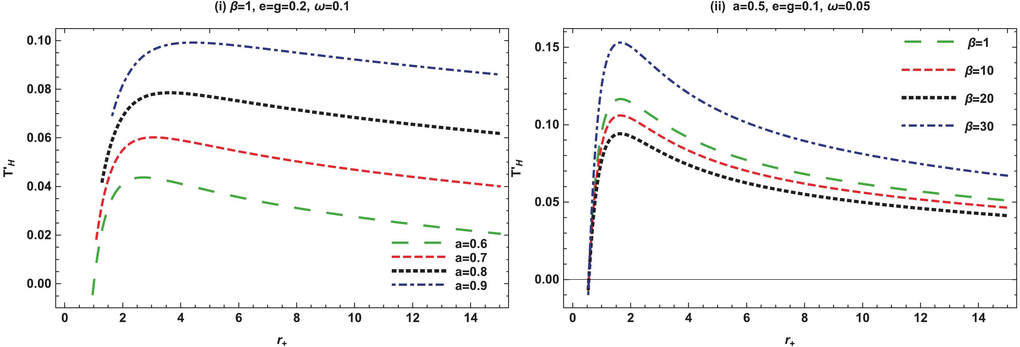
Figure 1. (color online)
$ T'_{H} $ vs.$ r_{+} $ for$ \alpha = 0.1 $ ,$ k = 0.5 $ &$ \ell = 0.4 $ .(i) An exponential increase in the temperature
$ T'_{H} $ is observed, and after attaining a height,$ T'_{H} $ slightly decreases with the increasing horizon$ r_{+} $ for varying values of the rotation parameter$ a $ . The$ T'_{H} $ decreases as the horizon increases, and this physical behavior reflects the BH stability with positive temperature untill$ r_{+}\rightarrow\infty $ . The temperature increases with the increase in$ a $ .(ii) We observe the behavior of the temperature for varying values of the correction parameter
$ \beta $ with fixed values of the other parameters. The$ T'_{H} $ decreases with increasing horizon in the domain$ 0\leqslant r_{+}\leqslant15 $ after attaining a maximum height. The maximum temperature with non-zero horizon reflects the BH remnant. This physical behavior of$ T'_{H} $ indicates the BH stability with a positive range. It is also worth notin that$ T'_{H} $ increases with the increase in correction parameter$ \beta $ .Figure 2 shows the behavior of
$ T'_{H} $ w.r.t$ r_{+} $ for fixed$ \alpha = 0.1 $ ,$ a = 0.5 $ &$ \ell = 0.4 $ .
Figure 2. (color online)
$ T'_{H} $ vs.$ r_{+} $ for$ \alpha = 0.1 $ ,$ a = 0.5 $ , &$ \ell = 0.4 .$ (i)
$ T'_{H} $ exponentially increases and slowly drops from a height for different values of electric and magnetic charges. The decrease in$ T'_{H} $ with the increasing horizon exhibits the stable state of BH in the domain$ 0\leqslant r_{+}\leqslant15 $ .$ T'_{H} $ decreases with the increase of BH electric and magnetic charges$ e $ and$ g $ , respectively.(ii) The temperature eventually drops down from a height for different values of the arbitrary parameter
$ k $ . There is a significant change in temperature as it decreases exponentially and attains an asymptotically flat shape, which indicates BH stability untill$ r_{+}\rightarrow+\infty $ . The$ T'_{H} $ increases with an increase of$ k $ .Figure 3 depicts the behavior of
$ T'_{H} $ w.r.t$ r_{+} $ for fixed$ a = 0.5 $ ,$ e = g = 5 $ &$ \ell = 0.4 $ for varying$ a $ and$ \omega $ in the domain$ 0\leqslant r_{+}\leqslant 5 $ .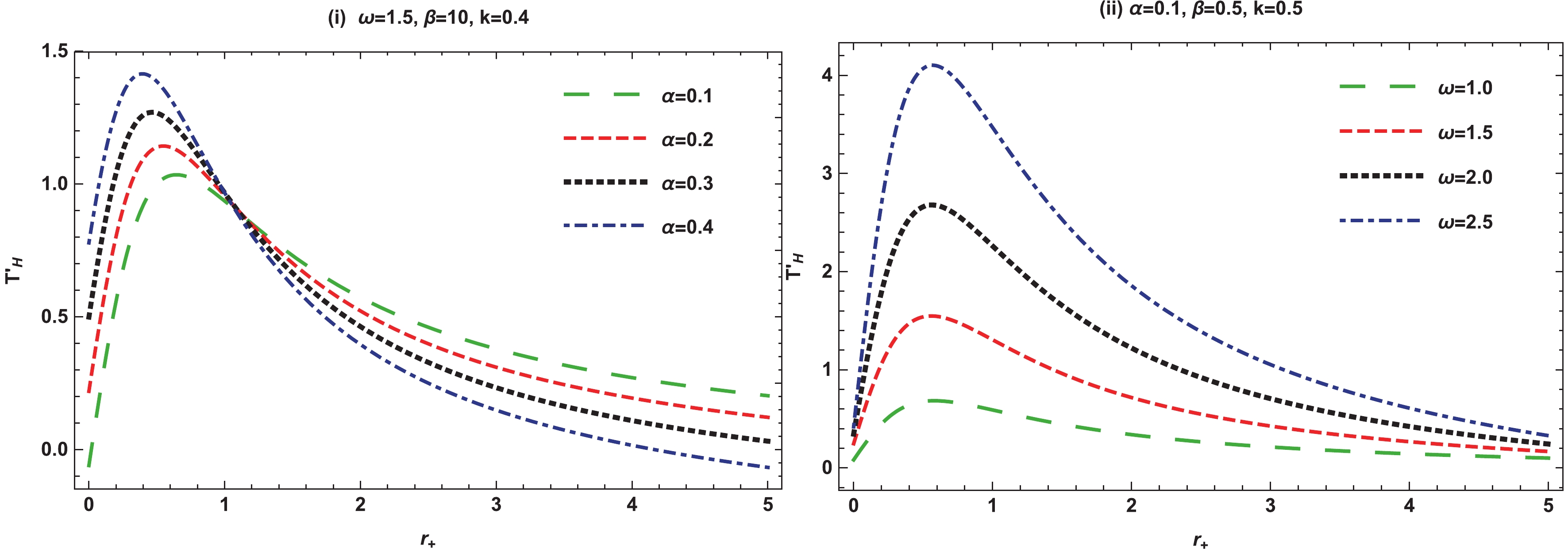
Figure 3. (color online)
$ T'_{H} $ vs.$ r_{+} $ for$ a = 0.5 $ ,$ e = g = 5 $ &$ \ell = 0.4. $ (i) Initially, the temperature increases with increasing horizon, and after a maximum height it exponentially decreases, which indicates the stable state of BH for different values of BH acceleration
$ \alpha $ .(ii) There can be seen that
$ T'_{H} $ exponentially increases and eventually drops from a height and decreases as the horizon increases untill$ r_{+}\rightarrow+\infty $ . This physical behavior indicates the stability of BH in positive ranges of different values of$ \omega $ . We observe that with the increase in the value of$ \omega $ ,$ T'_{H} $ increases. -
In this study, we have investigated the quantum gravity effects for vector bosons from charged accelerating rotating BH with the NUT parameter. By considering the GUP effects, we employed the modified Lagrangian equation incorporating quantum effects describing the motion of spin-1 particles. Subsequently, by applying the Hamilton-Jacobi technique, we have calculated the tunneling probabilities of vector bosons. Moreover, we analyzed the corrected Hawking temperatures of these BHs. We concluded that the modified tunneling probabilities are not just dependent on the BHs properties, but also on the properties of emitted vector bosons, i.e., energy, potential, surface gravity, particle charge, and total angular momentum. Moreover, it is important to note that the modified tunneling probabilities as well as the Hawking temperature depend on the quantum particles, which contribute gravitational radiation in form of massive particle (BH's energy carrier) tunneling.
When the quantum gravity effects are neglected, i.e.,
$ (\beta = 0) $ , then the corrected Hawking temperature Eq. (56) is reduced to the absolute temperature obtained by the quantum tunneling of vector bosons [78]. If we ignore the potential effects$ (A = 0) $ , the modified Hawking temperature is reduced to the temperature of vector (spin-1) particles provided in Refs. [69, 91]. Further, for$ \ell = 0 $ and$ \tilde{k} = 1 $ , the above results are reduced to the Hawking temperature of the accelerating and rotating BHs with electric and magnetic charges [85]. For$ \alpha = 0 $ , we recovered the temperature of non-accelerating BHs from the Hawking temperature of the charged accelerating and rotating BHs [86]. Moreover, for$ \beta = 0 $ ,$ \ell = 0 $ ,$ \tilde{k} = 1 $ and$ \alpha = 0 $ in Eq. (56), the Hawking temperature of the Kerr-Newman BH [87] is recovered, which is reduced for$ a = 0 $ to the temperature of the RN BH. For$ Q = 0 $ , the temperature reduces exactly to the Hawking temperature of the Schwarzschild BH at the residual mass of the BH [88].In our analysis, we have found that the quantum corrections decelerate the increase in temperature during the radiation process. This correction causes the radiation to cease at some specific temperature, leaving the remnant mass. The remnant mass is obtained at the specific condition
$ M_{\rm Res} \simeq \frac{M_{p}^2}{\beta_0\omega}\gtrsim \frac{M_{p}}{\beta_0}. $

(61) Here, it is important to mention that the value of the corrected Hawking temperature is smaller than the original Hawking temperature, and the BH stops radiating, when its mass reaches the minimal value
$ M_{\rm Res} $ . This result remains valid if the background BH geometry is more generalized.The results from the graphical analysis of corrected Hawking temperatures with respect to the horizon for the given BH are summarized as follows:
● For accelerating and rotating BH with NUT parameter, the
$ T'_{H} $ decreases with the increasing horizon, and BH reflects the stable state for varying values of the rotation parameter$ a $ and correction parameter$ \beta $ . The corrected temperature$ T'_{H} $ also increases with the increase in$ a $ and$ \beta $ . The BH remnant can be obtained at nonzero horizon with maximum temperature for different values of$ \beta $ in the domain$ 0\leqslant r_{+}\leqslant15 $ .● Corrected temperature
$ T'_{H} $ decreases with the increase of$ e $ and$ g $ . For different values of electric and magnetic charges, the BH exhibits stability in the domain$ 0\leqslant r_{+}\leqslant15 $ .● The
$ T'_{H} $ increases with the increase in the value of arbitrary parameter$ k $ .● The
$ T'_{H} $ increases with the increase in BH acceleration$ \alpha $ and rotation parameter$ \omega $ .● In our analysis, we considered the value
$ \Xi = 0.01 $ , then the condition of GUP must be satisfied for arbitrary values of$ 0\leqslant\beta<100 $ , the correction term is smaller than the usual term, and the positive temperature is obtained. For$ \beta>100 $ , the first order correction term becomes greater than the usual term, and the condition of GUP is not satisfied. Thus, we observe the negative temperature, which is non-physical. Furthermore, for$ \beta = 100 $ , the semi-classical term cancels out with the first order correction term, and hence the temperature vanishes.
Tunneling of massive vector particles under influence of quantum gravity
- Received Date: 2019-07-12
- Accepted Date: 2019-10-20
- Available Online: 2020-01-01
Abstract: This study set out to investigate charged vector particles tunneling via horizons of a pair of accelerating rotating charged NUT black holes under the influence of quantum gravity. To this end, we use the modified Proca equation incorporating generalized uncertainty principle. Applying the WKB approximation to the field equation, we obtain a modified tunneling rate and the corresponding corrected Hawking temperature for this black hole. Moreover, we analyze the graphical behavior of the corrected Hawking temperature


 DownLoad: