


 Abstract
 HTML
HTML Reference
 Related
 PDF
PDF


-
In the early 1920s, Kaluza and Klein attempted to establish a more fundamental theory that unifies the forces of electromagnetism and gravitation by introducing extra dimension(s) into general relativity [1]. The Kaluza-Klein (KK) theory attracted a lot of interest to explore extra dimensions in various observable phenomena [2–7]. In the middle of last century, this interest in extra dimensions has been enhanced because of the emergence of string/M theory, in which extra-dimensional spaces appear naturally. Inspired by the concept of brane in string theory [8], the braneworld scenario was proposed. This theory can efficiently explain some difficult problems in physics, such as the hierarchy problem (the electroweak scale/Higgs mass
$ M_{\rm EW}\sim1 $ TeV being significantly different from the Planck scale$ M_{\rm pl}\sim10^{16} $ TeV) and the cosmological constant problem [7,9–11].The most successful resolution of the hierarchy problem in the above theories is the Randall-Sundrum (RS) two-brane model [9]. The RS model takes into account the tension of the brane, which causes curving of the spacetime outside the brane. It consists of a 5D AdS bulk with a negative cosmological constant
$ \Lambda $ and a single extra dimension satisfying$ S1/Z_{2} $ orbifold symmetry. In such a scenario, our universe is described by a 5D metric$ \begin{array}{l} {\rm d}s^{2} = {\rm e}^{-2\sigma(\phi)}\eta_{\mu\nu}{\rm d}x^{\mu}{\rm d}x^{\nu}+r_{\rm c}^{2}{\rm d}\phi^{2}, \end{array} $

(1) where
$ \phi $ is the coordinate for an extra dimension,$ r_{\rm c} $ is the compactification radius,$ {\rm e}^{-2\sigma} $ is the warp factor with$ \sigma = kr_{\rm c}|\phi| $ , and$ k = \sqrt{-\Lambda/24M^{3}} $ with$ M $ denoting the 5D Planck mass. In this model, the weak scale is generated from the Planck scale through the warp factor, which originates from the background metric. However, the visible brane in the RS model exhibits negative tension, which is intrinsically unstable. Furthermore, the visible 3-brane (four-dimensional spacetime) has a zero cosmological constant, which is not consistent with the presently observed small value [11,12].This braneworld model has been widely studied. It was shown that the induced cosmological constant and the brane tension of the visible brane can be both positive or negative [13-15]. By replacing
$ \eta_{\mu\nu} $ with$ g_{\mu\nu} $ , a generalized RS braneworld scenario is achieved [11]. In this model, the negative brane cosmological constant is analyzed in detail [16-20]. It shows that$ N $ has a minimum value$ N_{\rm min} = 2n(n\approx16) $ , which leads to an upper bound for the induced negative cosmological constant. Furthermore, there are two different solutions to the hierarchical problem for a tiny cosmological constant. One solution corresponds to both the visible and hidden brane with positive tension. This is highly interesting, because both branes are stable. In another case, the induced positive cosmological constant corresponds to a negative tension visible brane, which is unstable, and not considered in the present study.In the above anti-de Sitter brane region, a large part of the parameter space corresponds to a positive value for the visible brane tension. However, our universe is currently undergoing accelerated expansion, which is indicated by recent observations of type Ia supernovae [21,22] and measurements of the anisotropies of the cosmic microwave background [23–25]. To explain this late-time epoch of accelerating expansion of the universe, we assume that there is a cosmological constant component in the 4D Einstein's field equation [26]. The cosmological constant is a very small value (
$ \simeq10^{-124} $ in Planck unit), which is restricted by the above experiments. Thus we need to cancel the induced negative cosmological constants to be consistent with observations.In this study, we focus on a 6D braneworld model, because there is no special reason to restrict the number of dimensions to five. For solving the above problem of the induced cosmological constant when the visible brane is negative, we consider the 4-brane (a extra dimension on the brane) in a 6D generalized RS model instead of the 3-brane in 5D generalized RS model. Subsequently, we obtain the effective induced positive cosmological constant of 4D spacetime with an anisotropic metric ansatz. At a little later period, the expansion of the 3D scale factor is as similar as the period of the radiation-dominated regime. Our study is organized as follows: In Sec. 2, by considering the 4-brane with the matter field Lagrangian in a 6D generalized RS model, we obtain a 5D Einstein field equation. In Sec. 3, we focus on the evolution of a 4-brane solved from the above field equation with an anisotropic metric ansatz. Finally, the summary and conclusion are presented in Sec. 4.
-
We start with a 6D generalized Randall-Sundrum model action:
$ \begin{array}{l} S = S_{\rm bulk}+S_{\rm vis}+S_{\rm hid} . \end{array} $

(2) The bulk action, visible brane action, and hidden brane action are respectively given by:
$ \begin{array}{l} S_{\rm bulk} = \int {\rm d}^{5}x{\rm d}y\sqrt{-G}(M^{4}_{6}R-\Lambda) , \end{array} $

(3) $ \begin{array}{l} S_{\rm vis} = \int {\rm d}^{5}x\sqrt{-g_{\rm vis}}({\cal{L}}_{\rm vis}-V_{\rm vis}), \end{array} $

(4) $ \begin{array}{l} S_{\rm hid} = \int {\rm d}^{5}x\sqrt{-g_{\rm hid}}({\cal{L}}_{\rm hid}-V_{\rm hid}), \end{array} $

(5) where
$ \Lambda $ is a bulk cosmological constant,$ M_{6} $ denotes the 6D fundamental mass scale,$ G_{AB} $ is the 6D metric tensor,$ R $ is the 6D Ricci scalar,$ {\cal{L}}_{\rm vis}({\cal{L}}_{\rm hid}) $ and$ V_{\rm vis}(V_{\rm hid}) $ are the matter field Lagrangian and the tension of the visible (hidden) brane, respectively.Variation of the above action with respect to the 6D metric tensor
$ G_{AB} $ led to Einstein’s equations:$ \begin{split} R_{AB}-\frac{1}{2}G_{AB}R =& \frac{1}{2M^{4}_{6}}\bigg\{-G_{AB}\Lambda+\sum_{i}[T^{i}_{AB} \times\delta(y-y_{i})\\&-G_{ab}\delta_{A}^{a}\delta_{B}^{b}V_{i}\delta(y-y_{i})]\bigg\}, \end{split} $

(6) where capital Latin
$ A,B $ indices ranging over all spacetime dimensions, lowercase Latin a,b = 0, 1, 2, 3, 4$ R_{AB} $ and$ T^{i}_{AB} $ are the 6D Ricci and the energy-momentum tensors respectively,$ y_{i} $ represents the position of the$ i $ -th brane in the sixth coordinate,$ i = {\rm hid} $ or$ {\rm vis} $ . The 6D stress-energy tensor$ T^{iA}_{B} $ is assumed to be that of an anisotropic perfect fluid and takes the form$ \begin{array}{l} T^{iA}_{B} = {\rm diag}[-\rho_{i}(t),p_{i1}(t),p_{i2}(t),p_{i3}(t),p_{i4}(t),0]. \end{array} $

(7) The metric ansatz in the generalized RS scenario, satisfying the 6D Einstein equations is
$ \begin{array}{l} {\rm d}s^{2} = G_{AB}{\rm d}x^{A}{\rm d}x^{B} = {\rm e}^{-2A(y)}g_{ab}{\rm d}x^{a}{\rm d}x^{b}+r^{2}{\rm d}y^{2}, \end{array} $

(8) where
$ g_{ab} $ is the 5D metric tensor. The corresponding Einstein equations are given by:$ \begin{array}{l} \widetilde{R} = {\rm e}^{-2A}\left(20A'^{2}+\displaystyle\frac{\Lambda}{M^{4}_{6}}\right), \end{array} $

(9) and
$ \begin{split} \widetilde{R}_{ab}-\frac{1}{2}g_{ab}\widetilde{R} =& g_{ab}{\rm e}^{-2A}\bigg\{(4A''-10A'^{2})-\frac{1}{2M^{4}_{6}}\bigg[\Lambda\\ &+\sum_{i}\delta(y-y_{i})V_{i}\bigg]\bigg\}+\frac{{\rm e}^{-2A}}{M^{4}_{6}}\sum_{i}T_{ab}^{i}\delta(y-y_{i}), \end{split} $

(10) where
$ \widetilde{R}_{ab} $ and$ \widetilde{R} $ are the 5D Ricci tensor and Ricci scalar respectively, defined with respect to$ g_{\mu\nu} $ . One side of Eq. (9) contains the derivatives of$ A(y) $ , depending on the extra coordinate$ y $ alone, while the other side depends on the brane coordinates$ x_{\mu} $ alone. Thus, each side is equal to an arbitrary constant. For convenience, we take this arbitrary constant to be$ 10\Omega/3 $ . Thus, we obtain from Eq. (9):$ \begin{aligned} {\rm e}^{-2A}\left(20A'^{2}+\frac{\Lambda}{M^{4}_{6}}\right) = \frac{10}{3}\Omega, \end{aligned} $

(11) and
$ \begin{array}{l} \widetilde{R} = \displaystyle\frac{10}{3}\Omega. \end{array} $

(12) Multiplying both sides of Eq. (10) by
$ g^{ab} $ , and rearranging the terms, we obtain:$ \begin{split} \widetilde{R} =& -\frac{2}{3}{\rm e}^{-2A}\bigg\{(4A''-10A'^{2})-\frac{1}{2M^{4}_{6}}\\ &\times\bigg[\Lambda+\sum_{i}\delta(y-y_{i})V_{i}\bigg]\bigg\}-\frac{{\rm e}^{-2A}}{3M^{4}_{6}}\sum_{i}T^{i}\delta(y-y_{i}), \end{split} $

(13) where
$ T^{i} = g^{ab}T^{i}_{ab} $ . Using Eqs. (11) and (12) to cancel$ A'^{2} $ and$ \widetilde{R} $ in Eq. (13), we obtain a simplified expression for$ A'' $ ,$ \begin{aligned} A'' = \displaystyle\frac{\Omega}{6}{\rm e}^{2A}+\displaystyle\frac{1}{8M^{4}_{6}}\sum_{i}\delta(y-y_{i})\left(V_{i}-\displaystyle\frac{T^{i}}{5}\right). \end{aligned} $

(14) The left side and the first term of the right side depend on the extra coordinate
$ y $ alone, while the other term appears only when the extra coordinate$ y = y_{i} $ . Thus, we obtain$ T^{i} = constant $ . For convenience, we define$ T^{i}\equiv5C_{i} $ , where the the$ C_{i} $ is a constant. Eq. (14) can be written as:$ \begin{aligned} A'' = \dfrac{\Omega}{6}{\rm e}^{2A}+\frac{1}{8M^{4}_{6}}\sum_{i}\delta(y-y_{i})(V_{i}-C_{i}). \end{aligned} $

(15) Rearranging Eq. (11), we obtain an expression for
$ A'^{2} $ :$ \begin{array}{l} A'^{2} = \dfrac{\Omega}{6}{\rm e}^{2A}+k^{2}, \end{array} $

(16) where
$ k^{2}\equiv-\Lambda/20M^{4}_{6}>0 $ (for Ads bulk i.e.$ \Lambda<0 $ ). We cancel the$ A'^{2} $ and$ A'' $ in Eq. (10) by Eqs. (15) and (16), then obtain:$ \begin{split} \widetilde{R}_{ab}-\frac{1}{2}g_{ab}\widetilde{R} =& -\Omega g_{ab}+\frac{1}{2M^{4}_{6}}\\& \times\sum_{i}(T_{ab}^{i}-g_{ab}C_{i})\delta(y-y_{i}). \end{split} $

(17) From the above equation, we can see that
$ T_{ab}^{i}-g_{ab}C_{i} = 0 $ , and subsequently we obtain$ \rho_{i} = -p_{i1} = -p_{i2} = -p_{i3} = -p_{i4} = -C_{i} $ . Thus, each stress-energy tensor$ T_{ab}^{i} $ is similar to a constant vacuum energy. This is consistent with the RS model [9] in which each 3-brane Lagrangian separated out a constant vacuum energy. We define the$ \mathcal{V}_{i}\equiv V_{i}-C_{i} $ . Thus, we obtain a 5D Einstein field equation:$ \begin{aligned} \widetilde{R}_{ab}-\frac{1}{2}g_{ab}\widetilde{R} = -\Omega g_{ab}, \end{aligned} $

(18) and the system of equations of
$ A(y)'' $ and$ A'^{2} $ :$ \begin{aligned} \left\{ \begin{aligned} &A'' = \dfrac{\Omega}{6}{\rm e}^{2A}+\frac{1}{8M^{4}_{6}}\sum_{i}\delta(y-y_{i}){\cal{V}}_{i}, \\ &A'^{2} = \dfrac{\Omega}{6}{\rm e}^{2A}+k^{2}. \\ \end{aligned} \right. \end{aligned} $

(19) The above corresponds to the induced cosmological constant
$ \Omega $ on the visible brane. For the induced brane cosmological constant$ \Omega>0 $ and$ \Omega<0 $ , the brane metric$ g_{ab} $ may correspond to dS-Schwarzschild and AdS-Schwarzschild spacetimes, respectively [27]. We first consider the induced negative cosmological constant on the visible brane, the the following solution for the warp factor is obtained:$ \begin{array}{l} A = -\ln[\omega\cosh(k|y|+C_{-})], \end{array} $

(20) where
$ \omega\equiv-\Omega/6k^{2} $ , and the constant$ C_{-} = \ln\displaystyle\frac{1-\sqrt{1-\omega^{2}}}{\omega} $ for considering the normalization of this factor at the orbifold fixed point$ y = 0 $ . In the limit$ \omega\sim0 $ , the RS solution$ A = ky $ can be recovered. This is consistent with the results in Ref. [11]. The other solution$ C_{-} = \ln\displaystyle\frac{1+\sqrt{1-\omega^{2}}}{\omega} $ is excluded, because the RS solution can not be recovered in the$ \omega^{2}\rightarrow0 $ limit.We can obtain the 5D effective theory from the original action Eq. (3). We focus on the curvature term from which we can derive the scale of gravitational interactions:
$ \begin{array}{l} S_{\rm eff}\supset\int {\rm d}^{5}x\int_{-\pi}^{\pi}{\rm d}y\sqrt{-g}M^{4}_{6}r{\rm e}^{-3A(kry)}\tilde{R}, \end{array} $

(21) where we only focus on the coefficient proportional to the 5D Ricci scalar
$ \tilde{R} $ . The Legendre term [28] is not proportional to$ \tilde{R} $ when the metric was substituted inside the action. Thus, we do not consider this term here. We can perform the$ y $ integral to obtain a 5D action. Hence, we obtain$ \begin{split} M^{3}_{5{\rm pl}} =& M^{4}_{6}\left[\frac{\omega^{6}}{12kc_{1}^{3}}({\rm e}^{3kr\pi}-1)+\frac{c_{1}^{3}}{12k}(1-{\rm e}^{-3kr\pi})\right.\\& \left.+\frac{3\omega^{4}}{4kc_{1}}({\rm e}^{kr\pi}-1)+\frac{3\omega^{2}c_{1}}{4k}(1-{\rm e}^{-kr\pi})\right], \end{split} $

(22) where
$ c_{1}\equiv1+\sqrt{1-\omega^{2}} $ . We find that if$ \omega^{6}\ll {\rm e}^{-3kr\pi} $ , then$ M_{5{\rm pl}} $ depends only weakly on$ r $ in the large$ kr $ limit. Hence, Eq. (22) can be simplified to$ \begin{array}{l} M^{3}_{5{\rm pl}} = \displaystyle\frac{2M^{4}_{6}}{3k}(1-{\rm e}^{-3kr\pi}). \end{array} $

(23) Thus, we can obtain
$ M^{3}\simeq2M^{4}_{6}/3k $ in the large$ kr $ limit. In this 4-brane model, the 5D components of the bulk metric is$ g^{\rm vis}_{ab} = G_{\mu\nu}(x^{a},y = r\pi) $ , and we obtain:$ \begin{array}{l} g^{\rm vis}_{ab} = g_{ab}{\rm e}^{-2A(kr\pi)}, \end{array} $

(24) $ \begin{array}{l} \sqrt{-g_{\rm vis}} = \sqrt{-g}{\rm e}^{-3A(kr\pi)}. \end{array} $

(25) From the above equations, we can not determine the physical masses by properly normalizing the fields, i.e., the hierarchy problem cannot be solved in this 4-brane model.
Taking the second derivative of Eq. (20) with respect to
$ y $ , we obtain:$ \begin{split} A'' =& \frac{\Omega}{6}{\rm e}^{2A}-2k\tanh\left(k|y|+\ln\frac{1-\sqrt{1-\omega^{2}}}{\omega}\right)\\& \times(\delta(y)-\delta(y-y_{\rm vis})). \end{split} $

(26) The orbifold fixed point
$ y_{\rm hid} = 0 $ . Comparing the above equation with Eq. (19), we obtain the tension of the visible (hidden)$ V_{\rm vis} $ ($ V_{\rm hid} $ ):$ \begin{aligned} V_{\rm vis} = 16M^{4}_{6}k\left[\frac{{\rm e}^{2kr\pi}\displaystyle\frac{\omega^{2}}{c_{1}^{2}}-1} {{\rm e}^{2kr\pi}\displaystyle\frac{\omega^{2}}{c_{1}^{2}}+1}\right], \end{aligned} $

(27) and
$ \begin{aligned} V_{\rm hid} = 16M^{4}_{6}k\left[\frac{1-\displaystyle\frac{\omega^{2}}{c_{1}^{2}}}{1+\displaystyle\frac{\omega^{2}}{c_{1}^{2}}}\right]. \end{aligned} $

(28) Setting
$ {\rm e}^{-A(r\pi)} = 10^{-n} $ , we then obtain from Eq. (20):$ \begin{array}{l} 10^{-N} = 4(10^{-n}{\rm e}^{-x}-{\rm e}^{-2x}), \end{array} $

(29) $ \begin{aligned} {\rm e}^{-x} = \frac{10^{-n}}{2}\left[1\pm\sqrt{1-10^{-(N-2n)}}\right], \end{aligned} $

(30) where
$ x\equiv\pi kr $ ,$ \omega^{2}\equiv10^{-N} $ . For$ 1-10^{2n}\omega^{2}\geqslant 0 $ , we find$ \omega^{2}\leqslant 10^{2n} $ , which leads to an upper bound for the cosmological constant ($ \sim10^{-N} $ ) given by$ N_{\rm min} = 2n $ . Eq. (30) has two values of$ x $ instead of one, and both values give rise to the required warping. For$ (N-2n)\gg1 $ , the first solution of$ x $ corresponds to the RS value plus a minute correction, which is given by$ x_{1} = n\ln10+\displaystyle\frac{1}{4}10^{-(N-2n)} $ , while the second solution of$ x $ is given by$ x_{2} = (N-n)\ln10+\ln4 $ [11]. Apparently, the$ x_{2} $ is greater than the$ x_{1} $ . Rewriting Eq. (27) with$ n $ and$ N $ , we obtain:$ \begin{aligned} {\cal{V}}_{\rm vis} = 16M^{4}_{6}k\frac{1-10^{N-2n}[1\pm\sqrt{1-10^{-(N-2n)}}]}{10^{N-2n}[1\pm\sqrt{1-10^{-(N-2n)}}]}, \end{aligned} $

(31) where the visible brane tension
$ {\cal{V}}_{\rm vis} $ is different from Eq. (23) derived in Ref. [11]. The two brane tensions are approximately given as:$ \begin{array}{l} {\cal{V}}_{\rm vis-1} = -16M^{4}_{6}k, \end{array} $

(32) $ \begin{array}{l} {\cal{V}}_{\rm vis-2} = 16M^{4}_{6}k. \end{array} $

(33) The visible brane tension in Eq. (33) is greater than Eq. (23) in Ref. [11], because the denominator of Eq. (31) is different from that of Eq. (23) in Ref. [11]. We see that a small negative cosmological constant suffices to render the tension positive, provided the distance between the branes is somewhat larger than the value predicted by the RS model. The tension
$ {\cal{V}}_{\rm vis-2} $ on the visible brane is inconsistent with Eq. (25) in Ref. [11]. Because of$ \omega\equiv10^{-N}\ll0 $ , we deduce that the hidden brane tension$ V_{\rm hid} $ is always positive.For
$ \Omega>0 $ , the warp factor that satisfies Eq. (19) is given by:$ \begin{array}{l} A = -\ln[\omega\sinh(-k|y|+C_{+})], \end{array} $

(34) where
$ \omega\equiv\Omega/6k^{2} $ ,$ C_{+} = \ln\displaystyle\frac{1+\sqrt{1+\omega^{2}}}{\omega} $ . In this case, the value of$ \omega^{2} $ is unbounded, such that the positive brane cosmological constant$ \Omega $ can be an arbitrary value. The solution of$ kr\pi $ provides a single solution instead of two solutions for$ \Omega<0 $ . Moreover, the above solution is dependent on$ \omega^{2} $ and$ n $ . For$ \Omega>0 $ , the visible brane tension$ {\cal{V}}_{\rm vis} $ and the hidden brane tension are always negative and positive, respectively [11]. The negative tension visible brane is unstable, and we do not consider this case. -
For
$ \Omega<0 $ , interestingly one can obtain the upper bound ($ \sim-10^{-2n} $ in Planck units) of the induced negative cosmological constant on the visible 4-brane. Meanwhile, the 4-brane tension can be positive for the second solution. In this study, we only consider two different spatial scaling factors$ a(t) $ and$ b(t) $ . -
First, we investigate the case with three
$ a(t) $ and one$ b(t) $ , which is mostly in line with the presently observed 3D space universe. We choose an anisotropic metric ansatz of the form$ g_{ab} = {\rm diag}[-1,a^{2}(t),a^{2}(t),a^{2}(t),b^{2}(t)] $ [26]. We allow the scale factor of the extra dimension on the visible brane$ b(t) $ to evolve at a rate different than that of the 3D scale factor$ a(t) $ . This metric describes a flat, homogeneous, and isotropic 3D space and a flat extra dimension of the visible brane. In this case, by adopting the above metric ansatz, we obtain the 5D Friedmann-Robertson-Walker (FRW) field equations from the Einstein field equations Eq. (18):$ \begin{array}{l} H_{a}^{2}+H_{a}H_{b} = \displaystyle\frac{1}{3}\Omega, \end{array} $

(35) $ \begin{array}{l} \dot{H}_{a}+2H_{a}^{2} = \displaystyle\frac{1}{3}\Omega, \end{array} $

(36) $ \begin{array}{l} 2\dot{H}_{a}+\dot{H}_{b}+3H_{a}^{2}+H_{b}^{2}+2H_{a}H_{b} = \Omega, \end{array} $

(37) where the dot denotes a time derivative, while
$ H_{a}\equiv\dot{a}/a $ and$ H_{b}\equiv\dot{b}/b $ are the Hubble parameters of the 3D space and extra dimension, respectively. Eq. (36) can thus be rewritten as:$ \begin{aligned} \frac{{\rm d}H_{a}}{H_{a}^{2}-\displaystyle\frac{1}{6}\Omega} = -2{\rm d}t. \end{aligned} $

(38) Upon integration of Eq. (36), we obtain the following solution for the 3D Hubble parameter:
$ \begin{array}{l} H_{a} = -\sqrt{-\displaystyle\frac{\Omega}{6}}\tan\left(2\sqrt{-\displaystyle\frac{\Omega}{6}}t+c\right), \end{array} $

(39) where
$ c $ is an arbitrary constant of integration. Performing the integration of Eq. (39), one finds the solution of 3D space scale factor$ a(t) $ :$ \begin{array}{l} a = c_{a}\left|\cos\left(2\sqrt{-\displaystyle\frac{\Omega}{6}}t+c\right)\right|^{\frac{1}{2}}, \end{array} $

(40) where
$ c_{a} $ is likewise an arbitrary constant of integration. We set that at the initial time$ t = 0 $ ,$ a = a_{0} $ . We can obtain$ c_{a} = a_{0}|\cos c|^{-\frac{1}{2}} $ , and Eq. (40) may then be rewritten as:$ \begin{aligned} a = a_{0}\frac{\left|\cos\left(2\sqrt{-\displaystyle\frac{\Omega}{6}}t+c\right)\right|^{\frac{1}{2}}}{|\cos c|^{\frac{1}{2}}}. \end{aligned} $

(41) where the scale factor
$ a(t) $ increases with the increasing of$ t $ when$ -\displaystyle\frac{\pi}{2}<2\sqrt{-\displaystyle\frac{\Omega}{6}}t+c<0 $ . For$ \Omega<0 $ , the induced negative cosmological constant is bounded from below by$ \sim-10^{-2n} $ . Assuming that the 3D space factor changes with time as smoothly as possible, we obtain the second solution$ x_{2}\simeq(N-n)\ln 10+\ln 4\simeq172 $ with$ n\simeq50 $ and$ N\simeq124 $ . Here, the above case$ n\simeq50 $ and$ N\simeq124 $ is satisfied in both conditions$ N-n\ll0 $ from$ \omega^{6}\ll {\rm e}^{-3kr\pi} $ and$ (N-2n)\gg1 $ . In this case of$ \Omega\simeq-10^{-124} $ , we obtain that$ 2\sqrt{-\displaystyle\frac{\Omega}{6}}t\ll1 $ when$ t $ is not very large (to date,$ t\sim10^{60} $ in Planck units). We set the constants$ c $ in Eq. (41) equal to$ -\pi/2 $ plus a small positive constant$ \chi $ to make sure that the scale factor$ a(t) $ is increasing from$ t = 0 $ to the present$ t\sim10^{60} $ . Then, the scale factor$ a(t) $ can be written:$ \begin{split} a =& a_{0}\frac{\left|\cos\left[2\sqrt{-\displaystyle\frac{\Omega}{6}}t-\displaystyle\frac{\pi}{2}+\chi\right]\right|^{\frac{1}{2}}}{\left|\cos \left(-\displaystyle\frac{\pi}{2}+\chi\right)\right|^{\frac{1}{2}}}\\ =& a_{0}\frac{\sin^{\frac{1}{2}}\left(2\sqrt{-\displaystyle\frac{\Omega}{6}}t+\chi\right)}{\sin^{\frac{1}{2}}\chi}. \end{split} $

(42) The Hubble parameter
$ H_{a} $ is rewritten as:$ \begin{split} H_{a} =& -\sqrt{-\displaystyle\frac{\Omega}{6}}\tan\left(2\sqrt{-\displaystyle\frac{\Omega}{6}}t-\displaystyle\frac{\pi}{2}+\chi\right)\\ =& \sqrt{-\displaystyle\frac{\Omega}{6}}\cot\left(2\sqrt{-\displaystyle\frac{\Omega}{6}}t+\chi\right). \end{split} $

(43) When
$ \sqrt{-\displaystyle\frac{\Omega}{6}}t\ll\chi\ll1 $ , the Hubble parameter$ H_{a} $ is obtained:$ \begin{array}{l} H_{a}\simeq\sqrt{-\displaystyle\frac{\Omega}{6}}\displaystyle\frac{1}{\chi}. \end{array} $

(44) Here,
$ H_{a} $ is a constant leading to an exponential expansion of the 3D scale factor. Comparing with the FRW equation in which the Gaussian curvature$ K = 0 $ , and with only the cosmological constant, we obtain the 4D effective cosmological constant$ \Lambda_{\rm eff} = -\Omega/2\chi^{2}>0 $ . However, the above period is so short that the 3D space scale factor only increases from$ a_{0} $ to$ a_{0}\left(1+\sqrt{\displaystyle\frac{-\Omega}{6\chi^{2}}}t\right) $ . After that, we obtain the Hubble parameter$ H_{a} $ and the 3D scale factor$ a(t) $ when$ \chi\ll\sqrt{-\displaystyle\frac{\Omega}{6}}t\ll1 $ :$ \begin{array}{l} H_{a}\simeq\displaystyle\frac{1}{2t} , \end{array} $

(45) $ \begin{array}{l} a(t)\simeq a_{0}\left(-\displaystyle\frac{2\Omega}{3\chi^2}\right)^{\frac{1}{4}}t^{\frac{1}{2}} , \end{array} $

(46) where
$ a(t) $ is proportional to$ t^{\frac{1}{2}} $ , which is as similar as the period of the radiation-dominated regime. The deceleration parameter$ q\equiv-\ddot{a}a/\dot{a}^{2} = 1-\Omega/3H_{a}^{2}>1 $ . This is unsatisfactory, because the aforementioned deceleration parameter is not consistent with the currently undergoing accelerated expansion.Using Eqs. (35) and (43), the extra dimension Hubble parameter
$ H_{b} $ is given by:$ \begin{split} H_{b} = &\frac{\Omega}{3H_{a}}-H_{a} = \frac{\Omega}{3\sqrt{-\displaystyle\frac{\Omega}{6}}\cot\left(2\sqrt{-\displaystyle\frac{\Omega}{6}}t+\chi\right)}\\ &-\sqrt{-\displaystyle\frac{\Omega}{6}}\cot\left(2\sqrt{-\displaystyle\frac{\Omega}{6}}t+\chi\right). \end{split} $

(47) When
$ H_{a}>0 $ , we obtain$ H_{b}<0 $ , and vice versa. Performing the integration of Eq. (47), one finds the solution of the extra dimension scale factor$ b(t) $ :$ \begin{aligned} b = b_{0}\frac{\sin^{\frac{1}{2}}\chi\cos\left(2\sqrt{-\displaystyle\frac{\Omega}{6}}t+\chi\right)}{\cos\chi\sin^{\frac{1}{2}}\left(2\sqrt{-\displaystyle\frac{\Omega}{6}}t+\chi\right)}, \end{aligned} $

(48) where we considered the initial conditions at time
$ t = 0 $ ,$ b = b_{0} $ . Form Eqs. (41) and (48), it is apparent that the scale factor$ a(t) $ and$ b(t) $ are impossible to increase or reduce at the same time. When the scale factor$ a(t) $ increases,$ b(t) $ decreases, and vice versa. Hence, the decrease of$ b(t) $ provides a driving force for the increasing of$ a(t) $ .The above investigation is the case of the increasing 3D scale factor
$ a(t) $ . In the following, we investigate the case where the scale factor$ a(t) $ decreases with the increasing of time$ t $ when$ 0<2\sqrt{-\displaystyle\frac{\Omega}{6}}t+c<\displaystyle\frac{\pi}{2} $ in Eq. (41). The analysis is similar to the previous one, as we substitute a small positive constant$ \psi $ into the constants$ c $ in Eq. (41). The Hubble parameter$ H_{a} $ and$ H_{b} $ are rewritten as:$ \begin{array}{l} H_{a} = -\sqrt{-\displaystyle\frac{\Omega}{6}}\tan\left(2\sqrt{-\displaystyle\frac{\Omega}{6}}t+\psi\right), \end{array} $

(49) $ \begin{split} H_{b} =& \frac{\Omega}{3H_{a}}-H_{a} = -\frac{\Omega}{\sqrt{-\displaystyle\frac{\Omega}{6}}\tan\left(2\sqrt{-\displaystyle\frac{\Omega}{6}}t+\psi\right)}\\ &-\sqrt{-\displaystyle\frac{\Omega}{6}}\tan\left(2\sqrt{-\displaystyle\frac{\Omega}{6}}t+\psi\right). \end{split} $

(50) Hence, we obtain the scale factors
$ a(t) $ and$ b(t) $ :$ \begin{array}{l} a = a_{0}\displaystyle\frac{\cos^{\frac{1}{2}}\left(2\sqrt{-\displaystyle\frac{\Omega}{6}}t+\psi\right)}{\cos^{\frac{1}{2}}\psi}, \end{array} $

(51) $ \begin{aligned} b = b_{0}\frac{\cos^{\frac{1}{2}}\psi\sin\left(2\sqrt{-\displaystyle\frac{\Omega}{6}}t+\psi\right)}{\sin\psi\cos^{\frac{1}{2}}\left(2\sqrt{-\displaystyle\frac{\Omega}{6}}t+\psi\right)}. \end{aligned} $

(52) When
$ \sqrt{-\displaystyle\frac{\Omega}{6}}t\ll\psi\ll1 $ , the Hubble parameter$ H_{a}\simeq-\sqrt{-\displaystyle\frac{\Omega}{6}}\psi $ is a negative constant. The Hubble parameter$ H_{b} $ is obtained:$ \begin{array}{l} H_{b}\simeq2\sqrt{-\displaystyle\frac{\Omega}{6}}\displaystyle\frac{1}{\psi}. \end{array} $

(53) Then we obtain the Hubble parameter
$ H_{b} $ and$ b(t) $ when$ \psi\ll\sqrt{-\displaystyle\frac{\Omega}{6}}t\ll1 $ :$ \begin{array}{l} H_{b}\simeq\displaystyle\frac{1}{t} , \end{array} $

(54) $ \begin{array}{l} b\simeq b_{0}\left(-\displaystyle\frac{2\Omega}{3\psi^2}\right)^{\frac{1}{2}}t , \end{array} $

(55) where
$ b(t) $ is proportional to$ t $ , which is faster than$ a(t) $ in the case of increasing$ a(t) $ . Because the decreasing of three dimensions instead of one provides dynamic. In Case I, the decreasing of scale factor(s) on the brane does (do) not provide sufficient impetus for the other scale factor(s) to expand exponentially. -
Similarly to Case I, we investigate the case with two
$ a(t) $ and two$ b(t) $ . We choose an anisotropic metric ansatz of the form$ g_{ab} = {\rm diag}[-1,a^{2}(t),a^{2}(t),b^{2}(t),b^{2}(t)] $ . The 5D FRW field equations are of the form:$ \begin{array}{l} H_{a}^{2}+4H_{a}H_{b}+H_{b}^{2} = \Omega, \end{array} $

(56) $ \begin{array}{l} \dot{H}_{a}+2\dot{H}_{b}+H_{a}^{2}+3H_{b}^{2}+2H_{a}H_{b} = \Omega, \end{array} $

(57) $ \begin{array}{l} \dot{H}_{b}+2\dot{H}_{a}+H_{b}^{2}+3H_{a}^{2}+2H_{a}H_{b} = \Omega. \end{array} $

(58) where
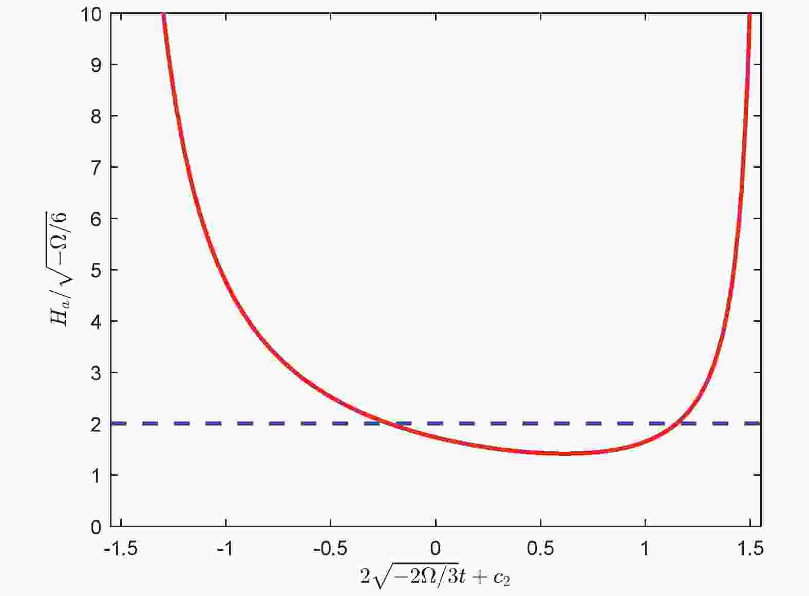
$ H_{a} $ and$ H_{b} $ are symmetric. Setting$ H_{a} $ positive and$ H_{b} $ negative, we obtain the following solutions for the Hubble parameters$ H_{a} $ and$ H_{b} $ , respectively:$ \begin{split} H_{a} =& -\sqrt{\displaystyle\frac{-\Omega}{6}}\left[\tan\left(2\sqrt{\displaystyle\frac{-2\Omega}{3}}t+c_{2}\right)\right.\\ &\left.-\sqrt{3}\left|\sec\left(2\sqrt{\displaystyle\frac{-2\Omega}{3}}t+c_{2}\right)\right|\right] , \end{split} $

(59) $ \begin{split} H_{b} =& -\sqrt{\displaystyle\frac{-\Omega}{6}}\left[\tan\left(2\sqrt{\frac{-2\Omega}{3}}t+c_{2}\right)\right.\\ &\left.+\sqrt{3}\left|\sec\left(2\sqrt{\displaystyle\frac{-2\Omega}{3}}t+c_{2}\right)\right|\right] . \end{split} $

(60) As shown in Fig. 1, the Hubble parameter
$ H_{a} $ is close to a constant$ H\simeq2 $ in a large region$ -0.8<2\sqrt{-2\Omega/3}t+c_{2}<1.2 $ . This is very different from the Case I, in which the Hubble parameter$ H_{a} $ is a constant in a very tiny interval$ \sqrt{-\displaystyle\frac{\Omega}{6}}t\ll\chi\ll1 $ . Considering the constraints in Eqs. (59) and (60) as in Case I,$ 2\sqrt{-\displaystyle\frac{2\Omega}{3}}t $ changes slowly with$ t $ when we set the second solution$ x_{2}\simeq(N-n)\ln 10+\ln 4\simeq172 $ with$ n\simeq50 $ and$ N\simeq124 $ . We obtain the 3D effective cosmological constant$ \Lambda_{\rm eff} = -2\Omega/3>0 $ , which is independent of the integral constant. This important result indicates that we can obtain an exponential expansion solution, which is consistent with our presently observed universe when we start from induced negative cosmological constants on the brane. Nevertheless, it is unsatisfactory, because the numbers of the expansion scale factor is two. However, this problem should be solved in a higher dimensional brane.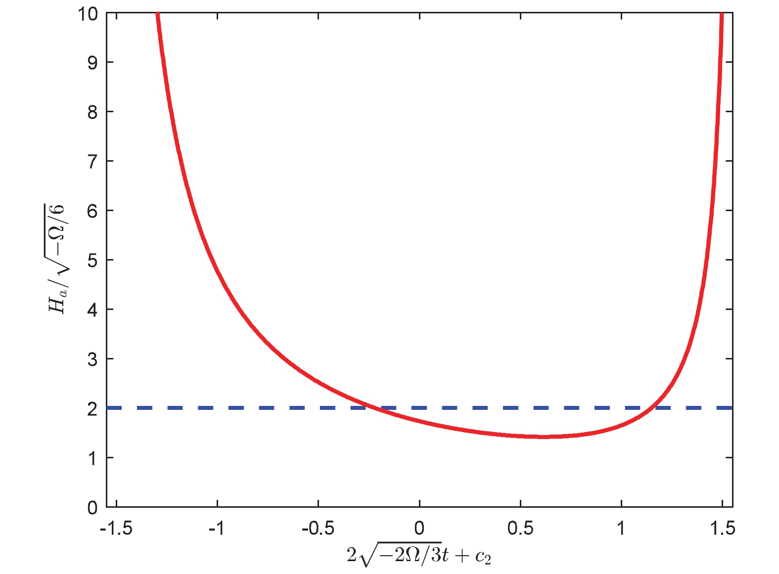
Figure 1. (color online) Hubble parameter
$H_{a}$ (solid curve) varies as a function of$2\sqrt{-2\Omega/3}t+c_{2}$ in Case II. The dashed curve depicts a constant$H\simeq2$ Finally, we consider an isotropic metric ansatz of the form
$ g_{ab} = {\rm diag}[-1,a^{2}(t),a^{2}(t),a^{2}(t),a^{2}(t)] $ in the 5D Einstein field equations Eq. (18), then we obtain the time-time component of 5D FRW field equations:$ \begin{array}{l} H_{a}^{2} = \displaystyle\frac{1}{6}\Omega. \end{array} $

(61) Here, no solution exists for the above equation, because
$ \Omega<0 $ . -
In this study, we investigate a 6D theory with a 4-brane to solve the cosmological fine-tuning problem. We find that each stress-energy tensor
$ T_{ab}^{i} $ on the brane is similar to a constant vacuum energy. The hierarchy problem cannot be solved efficiently in this model, which is consistent with the RS model [9], where each 3-brane Lagrangian yields a constant vacuum energy. The visible brane tension obtained in our study is greater than the result in Ref. [11]. For$ \Omega<0 $ , the induced negative cosmological constant on the visible 4-brane has an upper bound ($ \sim-10^{-32} $ in Planck units), and the 4-brane tension is positive for the second solution.In above case, we obtain the 5D FRW field equations from the Einstein field equations by adopting an anisotropic metric ansatz. In Case I, we find that the 3D space scale factor is increasing from
$ t = 0 $ to the present$ t\sim10^{60} $ . The constant Hubble parameter resulted in an exponential expansion of the 3D scale factor slightly after the initial time$ t = 0 $ . However, the period is so short that the 3D space scale factor only increases from$ a_{0} $ to$ a_{0}\left(1+\sqrt{\displaystyle\frac{-\Omega}{6\chi^{2}}}t\right) $ . When$ \chi\ll\sqrt{-\displaystyle\frac{\Omega}{6}}t\ll1 $ , the 3D space scale factor$ a(t) $ is proportional to$ t^{\frac{1}{2}} $ , which is similar to the period of the radiation-dominated regime.In Case II, we investigate the case with two
$ a(t) $ and two$ b(t) $ . In a large range of$ t $ , we obtain the 3D effective cosmological constant$ \Lambda_{\rm eff} = -2\Omega/3>0 $ , which is independent of the integral constant. Here, the scale factor is an exponential expansion, which is consistent with our presently observed universe. It is shown that the expansion rate of the scale factor is not directly related to the numbers of the scale factor of decrease. This is unsatisfactory, because there is two numbers for the expansion scale factor. However, this problem should be solved in a higher dimensional brane. Presently, it will be interesting to study whether the extra dimensions on the brane in this kind of generalized RS model with higher dimensions (e.g., 10D spacetime, as required by superstring theory) would provide enough impetus for 3D space exponential expansion. We hope to report these in future studies.
Anisotropic evolution of 4-brane in a 6D generalized Randall-Sundrum model
- Received Date: 2019-05-05
- Available Online: 2019-09-01
Abstract: We investigate a 6D generalized Randall-Sundrum brane world scenario with a bulk cosmological constant. Each stress-energy tensor


 DownLoad: