


 Abstract
 HTML
HTML Reference
 Related
 PDF
PDF


-
In recent years, three-body hadronic B/
$ B_s $ meson decays have attracted considerable attention of the experiments [1-3]. These processes provide new ways of studying the phenomenology of the Standard Model and of probing new physics effects. For instance, the LHCb collaboration has measured sizable direct CP asymmetries in the phase space of the three-body B decays [4, 5]. In addition, these processes are also valuable for understanding the mechanism of multi-body heavy meson decays.On the theoretical side, the perturbative QCD (PQCD) framework, based on the
$ k_T $ factorization, has been applied to analyze the B/$ B_s $ semi-leptonic and two-body decays processes [6-30]. The PQCD framework has also been used to study three-body decays [31-41]. Generally, the multi-scale decay amplitude may be written as a convolution, including the nonperturbative wave functions, hard kernel at the intermediate scale and short-distance Wilson coefficients. The factorization is greatly simplified if two of the final hadrons move collinearly. In this case, the three-body decays are reduced to quasi-two-body processes. Therefore, nonperturbative wave functions include two-meson light-cone distributions, which contain both resonant and nonresoant contributions. For instance, the measurement of$B_s\!\to\!J/\psi $ $ (\pi^+\pi^-)_S $ by LHCb [5] indicates that the resonances$ f_0(500) $ ,$f_0(980), f_0(1500), $ $ f_0(1790) $ of the S-wave$ \pi\pi $ -pair are dominant, which is confirmed by the theoretical calculation in the framework of PQCD [42-47]. In this work, we focus on$\bar B_s^0\to $ $ D^0(\bar D^0) \pi^+\pi^- $ and include the$ B_s \to D\, (f_0\,(500)+f_0\,(980)+ $ $f_0\,(1500)+f_0\,(1790) )\to D\,[(\pi^+\pi^-)_S] $ contributions. More explicitly, a Breit-Wigner (BW) model is used for the resonances$ f_0(500), f_0(1500),$ $ f_0(1790) $ [48] , and the Flatté model is adopted for the resonance$ f_0(980) $ [49].$ \bar B_s^0\to D^0(\bar D^0) \pi^+\pi^- $ , with the CP eigenstate containing the interference amplitude from$ b\to c\bar u s $ ($ b\to u\bar c s $ ), is sensitive to the angle$ \gamma $ of the CKM Unitarity Triangle, whose precise measurement is one of the primary objectives in flavour physics.The paper is organized as follow: in Sec. 2, we introduce the wave functions of
$ B_s $ , D and of the two pions. Sec. 3 contains our perturbative calculation within the PQCD framework. In Sec. 4, we give the numerical results, and a conclusion is presented in the last section. -
In general, the wave function
$ \Phi_{\alpha\beta} $ with Dirac indices$ \alpha,\beta $ can be decomposed into 16 independent components,$ I_{\alpha\beta},\gamma^{\mu}_{\alpha\beta},(\gamma^{\mu}\gamma^5)_{\alpha\beta},\gamma^5_{\alpha\beta},\sigma^{\mu\nu}_{\alpha\beta} $ . For the pseudoscalar$ B_s $ meson, the light-cone matrix element is defined as$ \begin{split} &\int_0^1 {\frac{{{\rm d^{\,4}}z}}{{{{(2\pi )}^4}}}} {{\rm e}^{{\rm i}{k_1} \cdot z}}\langle 0|{b_\alpha }(0){\bar q_\beta }(z)|{\bar B_s}({P_{{B_s}}})\rangle = \\&\quad \frac{i}{{\sqrt {2{N_c}} }}{\left\{ ({\not\!\! P_{{B_s}}} + {m_{{B_s}}}){\gamma _5}\left[{\phi _{{B_s}}}({k_1}) + \frac{{\not\! n - \not \!v}}{{\sqrt 2 }}{\bar \phi _{{B_s}}}({k_1})\right]\right\} _{\alpha \beta }},\end{split}$

(1) where the light-cone vectors are
$ {{n}} = (1,0,0_T) $ and$ {{v}} = (0,1,0_T) $ . The two independent parts of the$ B_s $ meson light-cone distribution amplitude obey the following normalization conditions:$\int {\frac{{{\rm d^4}{k_1}}}{{{{(2\pi )}^4}}}} {\phi _{{B_s}}}({k_1}) = \frac{{{f_{{B_s}}}}}{{2\sqrt {2{N_c}} }},\quad \int {\frac{{{\rm d^4}{k_1}}}{{{{(2\pi )}^4}}}} {\bar \phi _{{B_s}}}({k_1}) = 0,$

(2) where
$ f_{B_s} $ is the decay constant of$ B_s $ meson. Since the contribution of$ \bar{\phi}_{B_s}(k_1) $ is numerically small [28], we neglect it and keep only the$ \phi_{B_s}(k_1) $ part in the above equation. In the momentum space the light-cone matrix of$ B_s $ meson can be expressed as follows:${\Phi _{{B_s}}} = \frac{i}{{\sqrt {2{N_c}} }}({\not\!\!P_{{B_s}}} + {m_{{B_s}}}){\gamma _5}{\phi _{{B_s}}}({k_1}).$

(3) Usually, the hard part is independent of
$ k^+ $ or/and$ k^- $ , thus one can integrate one of them out from$ \phi_{B_s}(k^+,k^-,k_{\perp}) $ . With b as the conjugate space coordinate of$ k_{\perp} $ , we can express$ \phi_{B_s}(x,k_{\perp}) $ in the b-space by${\Phi _{{B_s}}}{(x,b)_{\alpha \beta }} = \frac{i}{{\sqrt {2{N_c}} }}{[({\not\!\! P_{{B_s}}} + {m_{{B_s}}}){\gamma _5}]_{\alpha \beta }}{\phi _{{B_s}}}(x,b),$

(4) where x is the momentum fraction of the light quark in
$ B_s $ meson. In this paper, we adopt the following expression for$ \phi_{B_s}(x,b) $ ${\phi _{{B_s}}}(x,b) = {N_{{B_s}}}{x^2}{(1 - x)^2}{\rm{exp}}\left[ - \frac{{m_{{B_s}}^2{x^2}}}{{2\omega _b^2}} - \frac{{{{({\omega _b}b)}^2}}}{2}\right],$

(5) where
$ N_{B_s} $ is the normalization factor, which is determined by the above equation with b = 0. In our calculation, we adopt$ \omega_b = (0.50\pm0.05) {\rm GeV} $ [9] and$ f_{B_s} = (0.228\pm$ $ 0.004) {\rm GeV} $ [10], from which we determine$ N_{B_s} = 63.02 $ .The wave function of the charmed D meson, treated as the heavy-light system, is defined by the light-cone matrix element as follows [11]:
$ \begin{split} &\int_0^1 {\frac{{{\rm d^{\,4}}z}}{{{{(2\pi )}^4}}}} {{\rm e}^{{\rm i}{k_2} \cdot z}}\langle 0|{\bar c_\alpha }(0){q_\beta }(z)|{\bar D^0}({P_D}))\rangle =\\&\quad - \frac{i}{{\sqrt {2{N_c}} }}{\left\{ ({\not \!\!P_D} + m_D^0){\gamma _5}{\phi _D}({k_2})\right\} _{\beta \alpha }},\end{split}$

(6) which satisfies the normalization
$\int {\frac{{{\rm d^4}{k_2}}}{{{{(2\pi )}^4}}}} {\phi _D}({k_2}) = \frac{{{f_D}}}{{2\sqrt {2{N_c}} }}.$

(7) Here,
$ f_D $ is the decay constant, and the chiral D meson mass is taken as$ m^0_D = \displaystyle\frac{m_D^2}{m_c+m_d} = m_D+{\cal O}(\Lambda) $ . For the numerical calculation, we adopt the parametrization [50],$\begin{split} {\phi _D}({x_2},{b_2}) = &\frac{{{f_D}}}{{2\sqrt {2{N_c}} }}6{x_2}(1 - {x_2})[1 + {C_D}(1 - 2{x_2})]\\&\times{\rm{exp}}\left[ - \frac{{\omega _D^2b_2^2}}{2}\right],\end{split}$

(8) where the free shape parameter
$ C_D $ is$ C_D = 0.5\pm0.1 $ [14], and$ f_D $ ,$ \omega_D $ read as$ f_D = 0.209\pm 0.002 $ [10] and$ \omega_D = 0.1 $ [14].The S-wave two-pion distribution amplitude is then given as [46]
$ \begin{split} \Phi _{\pi \pi }^{S-\rm wave} =& \frac{1}{{\sqrt {2{N_c}} }}[\not \!\!p{\Phi _{\pi \pi }}(z,\xi ,m_{\pi \pi }^2) + {m_{\pi \pi }}\Phi _{\pi \pi }^s(z,\xi ,m_{\pi \pi }^2) \\&+ {m_{\pi \pi }}(\not\! n\not\! v - 1)\Phi _{\pi \pi }^T(z,\xi ,m_{\pi \pi }^2)],\end{split}$

(9) where
$ z $ is the momentum fraction carried by the spectator positive quark,$ \Phi_{\pi\pi} $ ,$ \Phi_{\pi\pi}^s $ and$ \Phi_{\pi\pi}^T $ are twist-2 and twist-3 distribution amplitudes.$ m_{\pi\pi} $ is the invariant mass of the pion pair. We consider that the two-pion system moves in the n direction.$ \xi $ as the momentum fraction of$ \pi^+ $ in the pion pair. The asymptotic forms are parametrized as [51-53]$\begin{split} {\Phi _{\pi \pi }} =& \frac{{{F_s}(m_{\pi \pi }^2)}}{{2\sqrt {2{N_c}} }}{a_2}6z(1 - z)3(2z - 1),\;\\\Phi _{\pi \pi }^s =& \frac{{{F_s}(m_{\pi \pi }^2)}}{{2\sqrt {2{N_c}} }},\;\Phi _{\pi \pi }^T = \frac{{{F_s}(m_{\pi \pi }^2)}}{{2\sqrt {2{N_c}} }}(1 - 2z).\end{split}$

(10) Here,
$ F_s(m_{\pi\pi}^2) $ and$ a_2 $ are the timelike scalar form factor and the Gegenbauer coefficient, respectively. As a first approximation, the S-wave resonances used to parametrize$ F_s(m_{\pi\pi}^2) $ include both the resonant and nonresonant parts of the S-wave two-pion distribution amplitude. Therefore, we take into account$ f_0(980), $ $f_0(1500) $ and$ f_0(1790) $ in the$ s\bar s $ density operator, and$ f_0(500) $ in the$ u\bar u $ density operator:$\begin{split} F_s^{s\bar s}(m_{\pi \pi }^2) =& \frac{{{c_1}m_{{f_0}(980)}^2{{\rm e}^{{\rm i}{\theta _1}}}}}{{m_{{f_0}(980)}^2 - m_{\pi \pi }^2 - i{m_{{f_0}(980)}}({g_{\pi \pi }}{\rho _{\pi \pi }} + {g_{KK}}{\rho _{KK}})}}\\ & + \frac{{{c_2}m_{{f_0}(1500)}^2{{\rm e}^{{\rm i}{\theta _2}}}}}{{m_{{f_0}(1500)}^2 - m_{\pi \pi }^2 - i{m_{{f_0}(1500)}}{\Gamma _{{f_0}(1500)}}(m_{\pi \pi }^2)}}\\ & + \frac{{{c_3}m_{{f_0}(1790)}^2{{\rm e}^{{\rm i}{\theta _3}}}}}{{m_{{f_0}(1790)}^2 - m_{\pi \pi }^2 - i{m_{{f_0}(1790)}}{\Gamma _{{f_0}(1790)}}(m_{\pi \pi }^2)}},\\ F_s^{u\bar u}(m_{\pi \pi }^2) =& \frac{{{c_0}m_{{f_0}(500)}^2}}{{m_{{f_0}(500)}^2 - m_{\pi \pi }^2 - i{m_{{f_0}(500)}}{\Gamma _{{f_0}(500)}}(m_{\pi \pi }^2)}}. \end{split}$

(11) $ c_0 $ ,$ c_i $ and$ \theta_i $ ,$ i = 1,2,3 $ , are tunable parameters.$ m_S $ is the pole mass of the resonance, and$ \Gamma_S(m_{\pi\pi}) $ is the energy dependent width of the S-wave resonance which decays into two pions. For the contribution of$ f_0(980) $ , an anomalous structure was found around 980 MeV in the$ \pi^+\pi^- $ scattering [54, 55]. This was accompanied by the observation of a narrow anomaly (less than 100 MeV wide) in the S-wave phase shift associated with an enhancement in the$ (I = 0)~ K\bar K $ system at threshold. It was shown that the anomaly could be understood as a narrow two-channel resonance, which combines the$ \pi\pi $ and$ K\bar K $ channels [56]. Generally, the Breit-Wigner (BW) model can be applied to describe an unstable particle as an isolated resonance. Since the resonance$ f_0(980) $ is near the threshold of$ K\bar K $ of about 992 MeV, the model should be modified to include the coupled channels$ f_0(980)\to \pi\pi $ and$ f_0(980)\to K\bar K $ [56]. Therefore, the Breit-Wigner form proposed by Flatté and adopted widely in many studies of the$ \pi-\pi $ and$ K\bar K $ system is also used in this work. In the Flatté model, the phase space factors$ \rho_{\pi\pi} $ and$ \rho_{KK} $ are given as [48]$\begin{split} {\rho _{\pi \pi }} =& \frac{2}{3}\sqrt {1 - \frac{{4m_{{\pi ^ \pm }}^2}}{{m_{\pi \pi }^2}}} + \frac{2}{3}\sqrt {1 - \frac{{4m_{{\pi ^0}}^2}}{{m_{\pi \pi }^2}}} ,\\{\rho _{KK}} =& \frac{1}{2}\sqrt {1 - \frac{{4m_{{K^ \pm }}^2}}{{m_{\pi \pi }^2}}} + \frac{1}{2}\sqrt {1 - \frac{{4m_{{K^0}}^2}}{{m_{\pi \pi }^2}}} .\end{split}$

(12) -
According to the factorization theorem, the amplitude of a process can be calculated as an expansion in
$ \alpha_s(Q) $ and$ \Lambda/Q $ , where Q denotes a large momentum transfer, and$ \Lambda $ is a small hadronic scale. Usually, the factorization formula for the nonleptonic b-meson decays can be expressed as$\begin{split} A \sim & \int_0^1 {\rm d} {x_1} {\rm d} {x_2} {\rm d} {x_3}\int {{{\rm d}^2}} {{{b}}_1}{{\rm d}^2}{{{b}}_2}{{\rm d}^2}{{{b}}_3}\;C(t){\phi _B}({x_1},{{{b}}_1},t)\\& \times H({x_1},{x_2},{x_3},{{{b}}_1},{{{b}}_2},{{{b}}_3},t){\phi _2}({x_2},{{{b}}_2},t){\phi _3}({x_3},{{{b}}_3},t),\end{split}$

(13) where the Wilson coefficients and the typical scale t. The hard kernel
$ H(x_i,{b}_i, { t}) $ , representing b-quark decay sub-amplitude, and the nonperturbative meson wave function$ \phi_{i}(x_i,{b}_i, { t}) $ , describe the evolution from scale t to the lower hadronic scale$ \Lambda_{\rm QCD} $ . For a review of this approach, see Ref. [7].The effective Hamiltonian for
$ \bar B_s^0\to D^0(\bar D^0) \pi^+\pi^- $ is given as${{\cal H}_{\rm eff}} = \frac{{{G_F}}}{{\sqrt 2 }}{V_{Qb}}{V_{qs}}({C_1}{O_1} + {C_2}{O_2}),\;(Q = c,u,\;q = u,c),$

(14) with
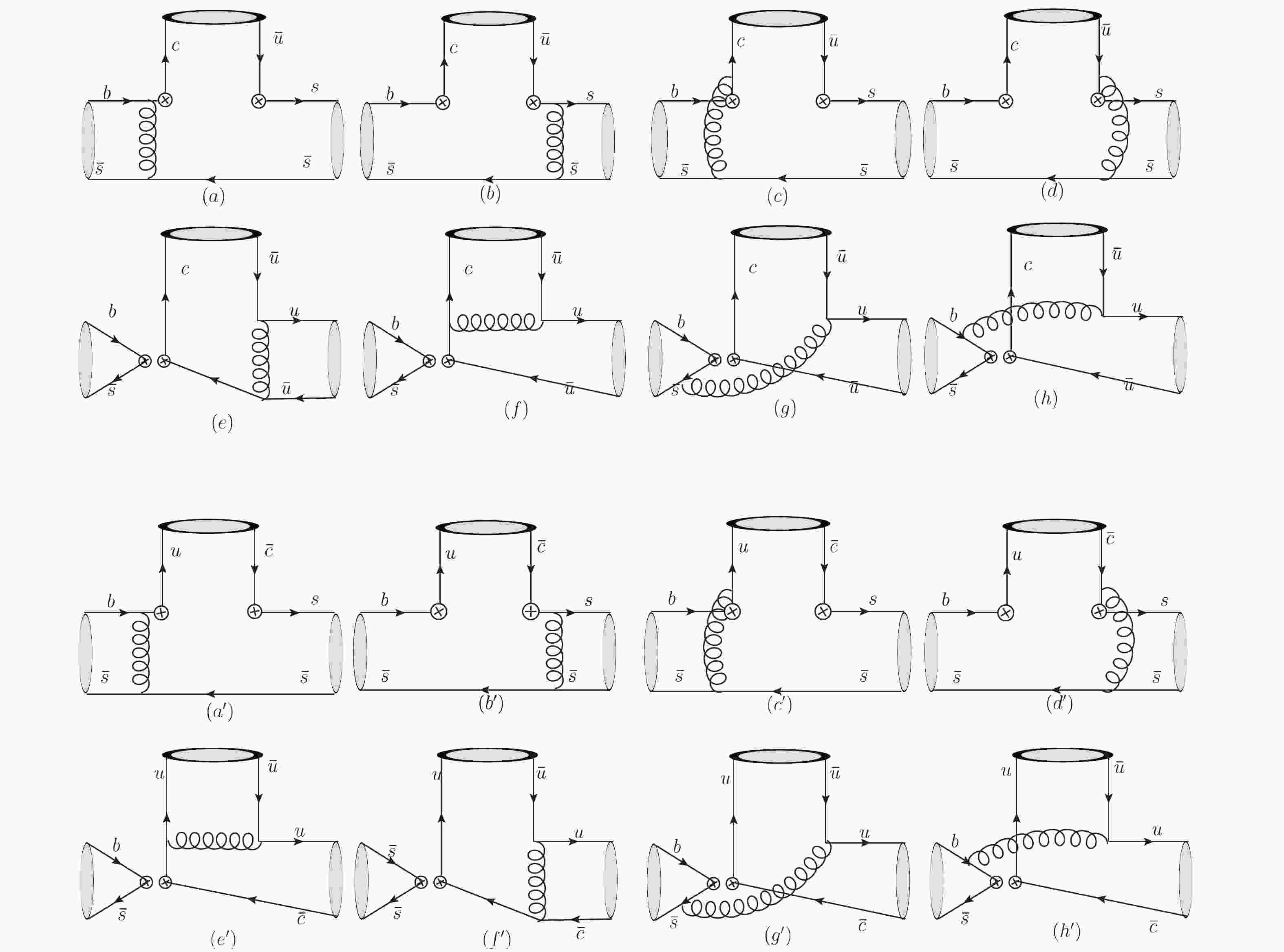
$ {O}_1 = (\bar c_{\alpha} b_{\beta})_{V-A}(\bar s_{\beta} u_{\alpha})_{V-A} $ ,$ {O}_2 = (\bar c_{\alpha} b_{\alpha})_{V-A}(\bar s_{\beta} u_{\beta})_{V-A} $ for the$ \bar B_s^0 \to D^0 \pi^+\pi^- $ process, and$ {O}_1 = (\bar u_{\alpha} b_{\beta})_{V-A}(\bar s_{\beta} c_{\alpha})_{V-A} $ ,$ {O}_2 = (\bar u_{\alpha} b_{\alpha})_{V-A}(\bar s_{\beta} c_{\beta})_{V-A} $ for the process$ \bar B_s^0 \to \bar D^0 \pi^+\pi^- $ . In particular, the penguin operators do not contribute to the processes. Using the above effective Hamiltonian, we obtain the typical Feynman diagrams for the$ \bar B_s^0 \to D^0 \pi^+\pi^- $ process shown in Fig. 1, in which the first row represents the color-suppressed emission process, and the second row indicates the W-exchange process. In the factorization framework, the factorizable diagrams in Fig. 1 (a,b,e,f) are relevant for$ a_2 $ , and the non-factorizable diagrams in Fig. 1 (c,d,g,h) are proportional to$ C_2 $ [57], where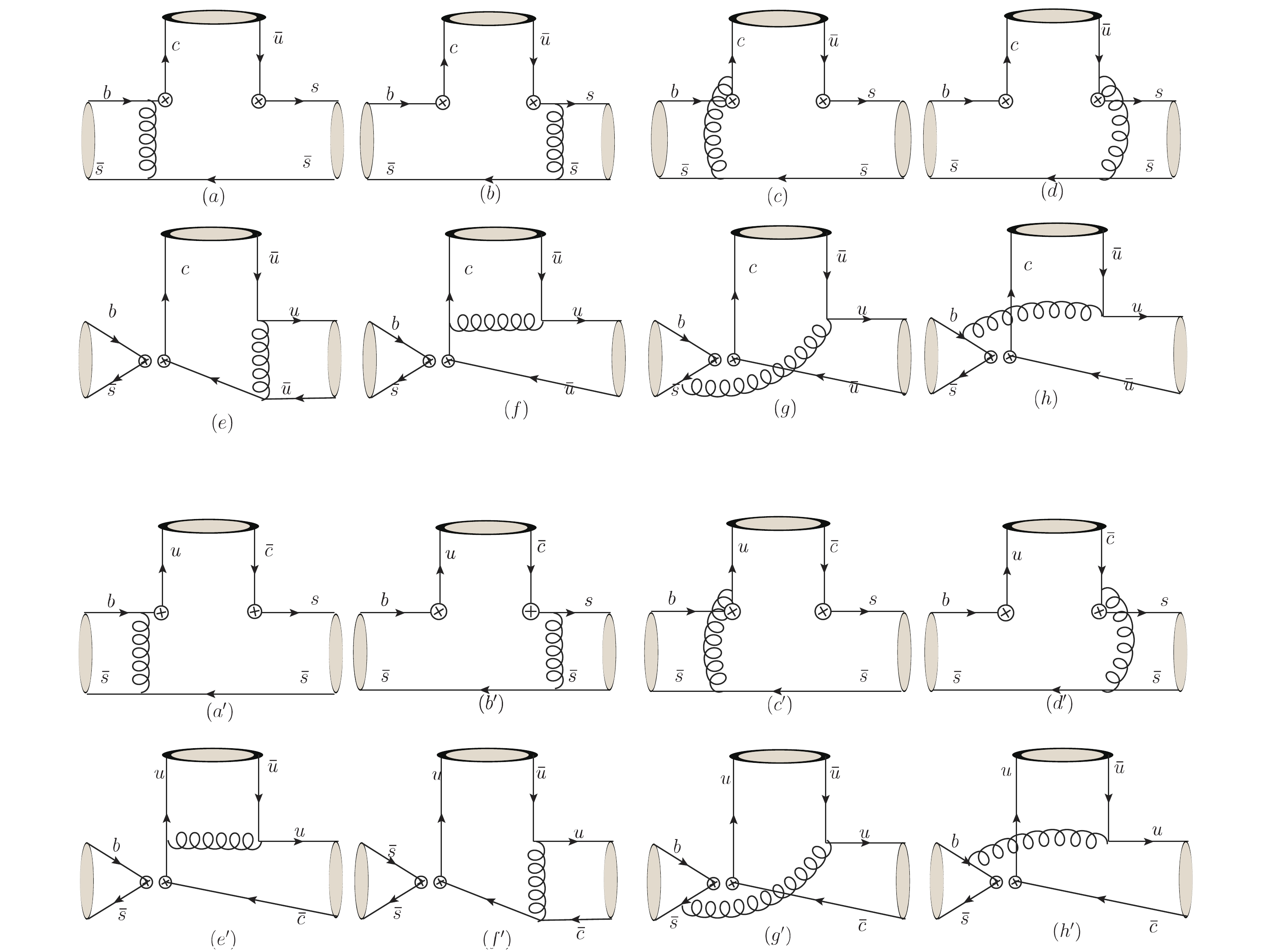
Figure 1. (color online) Typical Feynman diagrams for the three-body decays
$\bar B_s^0 \to D^0(\bar D^0)\pi^+\pi^-$ . For the three-body process, the operators at the quark level are${\cal O}_1, {\cal O}_2$ , which correspond to two kinds of Feynman diagrams: the color-suppressed and the W-exchange. The color-suppressed diagrams are shown in panels (a-d) and (a'-d'); the W-exchange diagrams are shown in panels (e-h) and (e'-h').${a_1} = {C_2} + {C_1}/{N_c},\quad {a_2} = {C_1} + {C_2}/{N_c}.$

(15) We will work in the light-cone coordinates. The momenta of the mesons are defined as follows:
$\begin{split} {P_{{B_s}}} =& (p_1^ + ,p_1^ - ,{0_ \bot }),\quad {P_{\pi \pi }} = (p_2^ + ,0,{0_ \bot }),\;\\{P_D} =& (p_1^ + - p_2^ + ,m_{{B_s}}^2/(2p_1^ + ),{0_ \bot }).\end{split}$

(16) Accordingly, the momentum transfer and the light-cone components can be obtained as
$q^2 = (P_{B_s}-P_{\pi\pi})^2 = $ $ (1-\rho)m_{B_s}^2 $ ,$ \rho = 1-\displaystyle\frac{m_D}{m_{B_s}} $ ,$ p_1^- = m_{B_s}^2/(2p_1^+) $ and$ p_2^+ = (m_{B_s}^2-$ $q^2)p_1^+/m_{B_s}^2 $ . In the heavy quark limit, the mass difference between b-quark (c-quark) and$ B_s(D) $ meson is negligible,$ m_{B_s,D} = m_{b,c} +\bar \Lambda $ ($ \bar \Lambda $ is of the order of the QCD scale). Since$ m_{B_s}\gg m_{D}\gg \bar \Lambda $ , we expand the amplitudes in terms of$ \displaystyle\frac{m_D}{m_{B_s}} $ ,$ \displaystyle\frac{\bar \Lambda}{m_D} $ , and for high order$ \displaystyle\frac{\bar \Lambda}{m_{B_s}} $ . For the leading order of the expansion,$ \rho\sim1, q^2\sim0 $ . The momenta of the light quarks in the mesons ($ k_1,k_3 $ represent the momenta of the light quarks in$ B_s $ and D mesons,$ k_2 $ is the momentum of the positive quark in the pion-pair system) are given as${k_1} = (0,{x_1}P_{{B_s}}^ - ,{k_{1 \bot }}),\;{k_2} = ({x_2}P_{\pi \pi }^ + ,0,{k_{2 \bot }}),\;{k_3} = (0,{x_3}P_D^ - ,{k_{3 \bot }}).$

(17) In the
$ k_T $ -factorization, the color-suppressed emission Feynman diagrams can be calculated out, with the formulas labeled as$ e_{x} $ (x = 1,2,3,4) in the subscript. Thus, the factorization formulas for the color-suppressed$ D^0 $ -emission diagrams are given as$\begin{split} {{\cal M}_{e12}} =& 8\pi {C_F}m_{{B_s}}^4{f_D}\int_0^1 {\rm d} {x_1}{\rm d}{x_2}\int_0^{1/\Lambda } {{b_1}}{\rm d}{b_1}{b_2}{\rm d}{b_2}{\phi _B}({x_1},{b_1})\\&\times\{ {E_{{e_1}}}({t_{{e_1}}}){h_{{e_1}}}({x_1},{x_2},{b_1},{b_2}){a_2}({t_{{e_1}}})\\ &\times[{r_0}(1 - 2{x_2})(\phi _{\pi \pi }^s(s\bar s,{x_2}) - \phi _{s\bar s,\pi \pi }^T({x_2})) \\&+ (2 - {x_2}){\phi _{\pi \pi }}(s\bar s,{x_2})] - 2{r_0}\phi _{\pi \pi }^s(s\bar s,{x_2})\\&\times{E_{{e_2}}}({t_{{e_2}}}){h_{{e_2}}}({x_1},{x_2},{b_1},{b_2}){a_2}({t_{{e_2}}})\} ,\\ {{\cal M}_{e34}} =& \displaystyle\frac{{32\pi {C_F}m_{{B_s}}^4}}{{\sqrt {2{N_c}} }}\int_0^1 {\rm d} {x_1}{\rm d}{x_2}{\rm d}{x_3}\int_0^{1/\Lambda } {{b_1}} {\rm d}{b_1}{b_3}{\rm d}{b_3}{\phi _B}({x_1},{b_1})\\&\times{\phi _D}({{\bar x}_3},{b_3}){C_2}({t_{{e_3}}})\{ {E_{{e_3}}}({t_{{e_3}}}){h_{{e_3}}}({x_1},{x_2},{x_3},{b_1},{b_3})\\&\times[{r_0}{{\bar x}_2}(\phi _{\pi \pi }^s(s\bar s,{x_2}) + \phi _{\pi \pi }^T(s\bar s,{x_2})) + {x_3}{\phi _{\pi \pi }}(s\bar s,{x_2})]\\ & - {E_{{e_4}}}({t_{{e_4}}}){h_{{e_4}}}({x_1},{x_2},{x_3},{b_1},{b_3})[{r_0}{{\bar x}_2}(\phi _{\pi \pi }^s(s\bar s,{x_2}) \\&- \phi _{\pi \pi }^T(s\bar s,{x_2})) + ({{\bar x}_3} + {{\bar x}_2}){\phi _{\pi \pi }}(s\bar s,{x_2})]\} , \end{split}$

(18) where
$ r_0 = \displaystyle\frac{m_{\pi\pi}}{m_{B_s}} $ ,$ C_F $ is the color factor.$ \phi_{\pi\pi}(s\bar s,x_2) $ represents the two-pion distribution amplitude defined by the$ s\bar s $ operator. The hard kernels$ E_{e_x} $ and$ h_{e_x} $ are given in the following.The factorization formulas for the W-exchange
$ D^0 $ diagrams$ {\cal M}_{w12} $ and$ {\cal M}_{w34} $ are given as$\begin{split} {{\cal M}_{w12}} =& 8\pi {C_F}m_{{B_s}}^4{f_{{B_s}}}\int_0^1 {\rm d} {x_2}{\rm d}{x_3}\int_0^{1/\Lambda } {{b_2}} {\rm d}{b_2}{b_3}{\rm d}{b_3}{\phi _D}({x_3},{b_3})\\&\times\{ {E_{{w_1}}}({t_{{w_1}}}){h_{{w_1}}}({x_2},{x_3},{b_2},{b_3}){a_2}({t_{{w_1}}})[{x_3}{\phi _{\pi \pi }}(u\bar u,{x_2}) \\&+ 2{r_0}{r_D}({x_3} + 1)\phi _{\pi \pi }^s(u\bar u,{x_2})] - [{x_2}{\phi _{\pi \pi }}(u\bar u,{x_2}) \\&- {r_0}{r_D}(2{x_2} + 1)\phi _{\pi \pi }^s(u\bar u,{x_2}) + {r_0}{r_D}(1\! -\! 2{x_2})\phi _{\pi \pi }^T(u\bar u,{x_2})]\\ &\times{E_{{w_2}}}({t_{{w_2}}}){h_{{w_2}}}({x_2},{x_3},{b_2},{b_3}){a_2}({t_{{w_2}}})\} ,\\ {{\cal M}_{w34}} =& \displaystyle\frac{{32\pi {C_F}m_{{B_s}}^4}}{{\sqrt {2{N_c}} }}\!\!\int_0^1 \!\!\!{\rm d} {x_1}{\rm d}{x_2}{\rm d}{x_3}\int_0^{1/\Lambda } \!\!\!{{b_1}} {\rm d}{b_1}{b_2}{\rm d}{b_2}{\phi _{{B_s}}}({x_1},{b_1}) \end{split}$

$\begin{split} &\times{\phi _D}({x_3},{b_2})\{ {E_{{w_3}}}({t_{{w_3}}}){h_{{w_3}}}({x_1},{x_2},{x_3},{b_1},{b_2}){C_2}({t_{{w_3}}})\\ &\times[{x_2}{\phi _{\pi \pi }}(u\bar u,{x_2}) + {r_0}{r_D}({x_2} + {x_3})\phi _{\pi \pi }^s(u\bar u,{x_2}) \\&+ {r_0}{r_D}({x_2} - {x_3})\phi _{\pi \pi }^T(u\bar u,{x_2})] + [ - {x_3}{\phi _{\pi \pi }}(u\bar u,{x_2}) \\ &- {r_0}{r_D}({x_2} + {x_3} + 2)\phi _{\pi \pi }^s(u\bar u,{x_2}) + {r_0}{r_D}({x_2} - {x_3})\\ &\times\phi _{\pi \pi }^T(u\bar u,{x_2})]{E_{{w_4}}}({t_{{w_4}}}){h_{{w_4}}}({x_1},{x_2},{x_3},{b_1},{b_2}){C_2}({t_{{w_4}}})\} , \end{split}$

(19) where
$ r_D = \displaystyle\frac{m_{D}}{m_{B_s}} $ ,$ \phi_{\pi\pi}(u\bar u,x_2) $ represents the distribution amplitude of the$ u\bar u $ operator. Due to the helicity suppression, the contribution of the factorizable diagrams$ {\cal M}_{w12} $ is suppressed significantly. Therefore, the dominant contribution comes from the non-factorizable diagrams$ {\cal M}_{w34} $ .In the
$ \bar D^0 $ -emission process, the two factorizable diagrams have the same factorization$ {\cal M}_{e12} = {\cal M}_{e'12} $ . Accordingly, we give the factorization formulas for the non-factorizable emission diagrams$ {\cal M}_{e'34} $ , the factorizable W-exchange diagrams$ {\cal M}_{w'12} $ and the non-factorizable W-exchange diagrams$ {\cal M}_{w'34} $ as follows:$\begin{split} {{\cal M}_{e'34}} =& \frac{{32\pi {C_F}m_{{B_s}}^4}}{{\sqrt {2{N_c}} }}\!\!\int_0^1 \!\!{\rm d} {x_1}{\rm d} {x_2}{\rm d}{x_3}\!\!\int_0^{1/\Lambda } \!\!{{b_1}}{\rm d}{b_1}{b_3}{\rm d}{b_3}{\phi _B}({x_1},{b_1})\\ &\times{\phi _D}({{\bar x}_3},{b_3})\{ {E_{{{e'}_3}}}({t_{{{e'}_3}}}){h_{{{e'}_3}}}({x_1},{x_2},{x_3},{b_1},{b_3}){C_2}({t_{{{e'}_3}}})\\ &\times[{r_0}({{\bar x}_2})(\phi _{\pi \pi }^s(s\bar s,{x_2}) + \phi _{\pi \pi }^T(s\bar s,{x_2})) + {x_3}{\phi _{\pi \pi }}(s\bar s,{x_2})]\\ & - \!{E_{{{e'}_4}}}({t_{{{e'}_4}}}){h_{{{e'}_4}}}({x_1},{x_2},{x_3},{b_1},{b_3}){C_2}({t_{{{e'}_4}}})[{r_0}{{\bar x}_2}(\phi _{\pi \pi }^s(s\bar s,{x_2}) \\ &- \phi _{\pi \pi }^T(s\bar s,{x_2})) + ({{\bar x}_3} + {{\bar x}_2}){\phi _{\pi \pi }}(s\bar s,{x_2})]\} ,\\ {{\cal M}_{w'12}} =& 8\pi {C_F}m_{{B_s}}^4{f_{{B_s}}}\int_0^1 {\rm d} {x_2}{\rm d}{x_3}\int_0^{1/\Lambda } {{b_2}} {\rm d}{b_2}{b_3}{\rm d}{b_3}{\phi _{\bar D}}({x_3},{b_3})\\ &\times\{ {E_{{{w'}_1}}}({t_{{{w'}_1}}}){h_{{{w'}_1}}}({x_2},{x_3},{b_2},{b_3}){a_2}({t_{{{w'}_1}}})\\ &\times[(1 - {x_2}){\phi _{\pi \pi }}(u\bar u,{x_2}) + {r_0}{r_D}(2{x_2} - 3)\phi _{\pi \pi }^s(u\bar u,{x_2}) \\ &+ {r_0}{r_D}(1 - 2{x_2})\phi _{\pi \pi }^T(u\bar u,{x_2})]+ [ - {x_3}{\phi _{\pi \pi }}(u\bar u,{x_2}) \\ & + 2{r_0}{r_D}({x_3} + 1)\phi _{\pi \pi }^s(u\bar u,{x_2})]{E_{{{w'}_2}}}({t_{{{w'}_2}}})\\ & \times{h_{{{w'}_2}}}({x_2},{x_3},{b_2},{b_3}){a_2}({t_{{{w'}_2}}})\} ,\\ {{\cal M}_{w'34}} =& \frac{{32\pi {C_F}m_{{B_s}}^4}}{{\sqrt {2{N_c}} }}\!\!\int_0^1 \!\!{\rm d} {x_1}{\rm d}{x_2}{\rm d}{x_3}\!\!\int_0^{1/\Lambda } \!\!{{b_1}} {\rm d}{b_1}{b_2}{\rm d}{b_2}{\phi _{{B_s}}}({x_1},{b_1})\\ & \times{\phi _{\bar D}}({x_3},{b_2})\{ {E_{{{w'}_3}}}({t_{{{w'}_3}}}){h_{{{w'}_3}}}({x_1},{x_2},{x_3},{b_1},{b_2}){C_2}({t_{{{w'}_3}}})\\ &\times[{x_3}{\phi _{\pi \pi }}(u\bar u,{x_2}) - {r_0}{r_D}(1 - {x_2} + {x_3})\phi _{\pi \pi }^s(u\bar u,{x_2})\\ & + {r_0}{r_D}({x_2} + {x_3} - 1)\phi _{\pi \pi }^T(u\bar u,{x_2})] + [({x_2} - 1){\phi _{\pi \pi }}(u\bar u,{x_2})\\ & + {r_0}{r_D}( - {x_2} + {x_3} + 3)\phi _{\pi \pi }^s(u\bar u,{x_2}) + {r_0}{r_D}({x_2} + {x_3} - 1)\\ & \times\phi _{\pi \pi }^T(u\bar u,{x_2})]{E_{{{w'}_4}}}({t_{{{w'}_4}}}){h_{{{w'}_4}}}({x_1},{x_2},{x_3},{b_1},{b_2}){C_2}({t_{{{w'}_4}}})\} . \end{split}$

(20) In the following, we give the forms for the offshellness of the intermediate gluon
$ \beta_{e_x} $ /$ \beta_{w_x} $ and quarks$ \alpha_{e_x} $ /$ \alpha_{w_x} $ ($ x = 1,2,3,4 $ ) in the$ \bar B_s^0 \to D^0 \pi^+\pi^- $ process.$\begin{split} {\alpha _{{e_1}}} =& (1 - {x_2})m_{{B_s}}^2\rho ,\;\;{\alpha _{{e_2}}} = {x_1}m_{{B_s}}^2\rho ,\;\;\\{\alpha _{{e_3}}} =& {x_1}(1 - {x_2})m_{{B_s}}^2\rho ,\;\;{\alpha _{{e_4}}} = {x_1}(1 - {x_2})m_{{B_s}}^2\rho ,\\ {\alpha _{{w_1}}} =& {x_3}m_{{B_s}}^2\rho ,\;\;{\alpha _{{w_2}}} = (1 - \rho + {x_2}\rho )m_{{B_s}}^2,\;\\{\alpha _{{w_3}}} =& {x_2}{x_3}m_{{B_s}}^2\rho ,\;\;{\alpha _{{w_4}}} = {x_2}{x_3}m_{{B_s}}^2\rho ,\\ {\beta _{{e_1}}} =& {x_1}(1 - {x_2})m_{{B_s}}^2\rho ,\;\;{\beta _{{e_2}}} = {x_1}(1 - {x_2})m_{{B_s}}^2\rho ,\;\\ {\beta _{{e_3}}} =& [({x_1} - {x_3})(1 - {x_2}\rho ) + (1 - \rho )]m_{{B_s}}^2,\;\\{\beta _{{e_4}}} =& (1 - {x_2})({x_1} + {x_3} - 1)m_{{B_s}}^2\rho ,\\ {\beta _{{w_1}}} =& {x_2}{x_3}m_{{B_s}}^2\rho ,\;\;{\beta _{{w_2}}} = {x_2}{x_3}m_{{B_s}}^2\rho ,\;\\ {\beta _{{w_3}}} =& ({x_3} - {x_1}){x_2}m_{{B_s}}^2\rho ,\;\\{\beta _{{w_4}}} =& ((1 - {x_1} - {x_3})(1 - {x_2}\rho ) - 1)m_{{B_s}}^2. \end{split}$

(21) For
$ B_s^0 \to \bar D^0 \pi^+\pi^- $ , we have$\begin{split} {\alpha _{{{e'}_1}}} =& (1 - {x_2})m_{{B_s}}^2\rho ,\;\;{\alpha _{{{e'}_2}}} = {x_1}m_{{B_s}}^2\rho ,\;\\{\alpha _{{{e'}_3}}} =& {x_1}(1 - {x_2})m_{{B_s}}^2\rho ,\;\;{\alpha _{{{e'}_4}}} = {x_1}(1 - {x_2})m_{{B_s}}^2\rho ,\\ {\alpha _{{{w'}_1}}} =& (1 - {x_2}\rho )m_{{B_s}}^2,\;\;{\alpha _{{{w'}_2}}} = {x_3}m_{{B_s}}^2\rho ,\\{\alpha _{{{w'}_3}}} = &{x_3}(1 - {x_2})m_{{B_s}}^2\rho ,\;\;{\alpha _{{{w'}_4}}} = {x_3}(1 - {x_2})m_{{B_s}}^2\rho ,\\ {\beta _{{{e'}_1}}} =& {x_1}(1 - {x_2})m_{{B_s}}^2\rho ,\;\;{\beta _{{{e'}_2}}} = {x_1}(1 - {x_2})m_{{B_s}}^2\rho ,\\ {\beta _{{{e'}_3}}} =& (1 - {x_2})({x_1} - {x_3})m_{{B_s}}^2\rho ,\\{\beta _{{{e'}_4}}} =& [({x_1} + {x_3} - 1)(1 - {x_2}\rho ) + (1 - \rho )]m_{{B_s}}^2,\\ {\beta _{{{w'}_1}}} =& {x_3}(1 - {x_2})m_{{B_s}}^2\rho ,\;\;{\beta _{{{w'}_2}}} = {x_3}(1 - {x_2})m_{{B_s}}^2\rho ,\\ {\beta _{{{w'}_3}}} =& (1 - {x_2})({x_3} - {x_1})m_{{B_s}}^2\rho ,\\{\beta _{{{w'}_4}}} =& ((1 - {x_1} - {x_3})(1 - \rho + {x_2}\rho ) - 1)m_{{B_s}}^2. \end{split}$

(22) The hard kernel functions
$ h_{e_x} $ ($ h_{e'_x} $ ) and$ h_{w_x} $ ($ h_{w'_x} $ ) are written as$\begin{split} {h_{{e_i}}}({x_1},{x_2},{b_1},{b_2}) =& [\theta ({b_1} - {b_2}){I_0}(\sqrt {{\alpha _{{e_i}}}} {b_2}){K_0}(\sqrt {{\beta _{{e_i}}}} {b_1}) + ({b_1} \leftrightarrow {b_2})]{K_0}(\sqrt {{\beta _{{e_i}}}} {b_1}){S_t}({\alpha _{{e_i}}}/(m_{{B_s}}^2\rho )),\\ {h_{{e_j}}}({x_1},{x_2},{x_3},{b_1},{b_3}) =& [\theta ({b_1} - {b_3}){I_0}\left(\sqrt {{\alpha _{{e_j}}}} {b_3}\right){K_0}\left(\sqrt {{\beta _{{e_j}}}} {b_1}\right) + ({b_1} \leftrightarrow {b_3})] \left\{ {\begin{array}{*{20}{l}} {{K_0}\left(\sqrt {{\beta _{{e_j}}}} {b_1}\right),}&{{\beta _{{e_j}}} \geqslant 0,}&{}\\ {\displaystyle\frac{{i\pi }}{2}H_0^{(1)}\left(\sqrt {|{\beta _{{e_j}}}|} {b_1}\right),}&{{\beta _{{e_j}}} < 0,}&{} \end{array}} \right.,\\ {h_{{w_k}}}({x_1},{x_2},{b_2},{b_3}) =& {\left(i\displaystyle\frac{\pi }{2}\right)^2}H_0^{(1)}(\sqrt {{\beta _{{w_k}}}} {b_2})[\theta ({b_2} - {b_3})H_0^{(1)}(\sqrt {{\alpha _{{w_k}}}} {b_2}){J_0}(\sqrt {{\alpha _{{w_k}}}} {b_3}) + ({b_2} \leftrightarrow {b_3})]{S_t}({\alpha _{{w_k}}}/(m_{{B_s}}^2\rho )),\\ {h_{{w_l}}}({x_1},{x_2},{x_3},{b_1},{b_2}) =& i\frac{\pi }{2}[\theta ({b_1} - {b_2})H_0^{(1)}(\sqrt {{\alpha _{{w_l}}}} {b_1}){J_0}(\sqrt {{\alpha _{{w_l}}}} {b_2}) + ({b_1} \leftrightarrow {b_2})] \left\{ {\begin{array}{*{20}{l}} {{K_0}(\sqrt {{\beta _{{w_l}}}} {b_1}),}&{{\beta _{{w_l}}} \leqslant 0,}&{}\\ {\displaystyle\frac{{i\pi }}{2}H_0^{(1)}(\sqrt {|{\beta _{{w_l}}}|} {b_1}),}&{{\beta _{{w_l}}} > 0,}&{} \end{array}} \right.. \end{split}$

(23) where
$ i,k = 1,2 $ and$ j,l = 3,4 $ , and$ I_0 $ ,$ K_0 $ and$ H_0 = J_0+i Y_0 $ are the Bessel functions. The threshold re-summation factor$ S_t(x) $ is parametrized as${S_t}(x) = \frac{{{2^{1 + 2c\Gamma (3/2 + c)}}}}{{\sqrt \pi \Gamma (1 + c)}}{[x(1 - x)]^c},$

(24) with the parameter
$ c = 0.4 $ in this work. The evolution factors$ E_{x}(t) $ in the factorization formulas are given by$\begin{split} {E_{{e_i}}}(t) =& {\alpha _s}(t){\rm{exp}}( - {S_{{B_s}}}(t) - {S_{\pi \pi }}(t)),\\ {E_{{e_j}}}(t) =& {\alpha _s}(t){\rm{exp}}( - {S_{{B_s}}}(t) - {S_{\pi \pi }}(t) - {S_D}(t)){|_{{b_1} = {b_2}}},\\ {E_{{w_k}}}(t) =& {\alpha _s}(t){\rm{exp}}( - {S_{\pi \pi }}(t) - {S_D}(t)),\\ {E_{{w_l}}}(t) = &{\alpha _s}(t){\rm{exp}}( - {S_{{B_s}}}(t) - {S_{\pi \pi }}(t) - {S_D}(t)){|_{{b_2} = {b_3}}}, \end{split}$

(25) where
$\begin{split} {S_{{B_s}}}(t) = s({x_1}{m_{{B_s}}},{b_1}) + \frac{5}{3}\int_{1/{b_1}}^t {\frac{{\rm d\bar \mu }}{{\bar \mu }}} {\gamma _q}({\alpha _s}(\bar \mu )), \end{split}$

$\begin{split} {S_D}(t) =& s({x_3}{m_{{B_s}}},{b_3}) + 2\int_{1/{b_3}}^t {\frac{{\rm d\bar \mu }}{{\bar \mu }}} {\gamma _q}({\alpha _s}(\bar \mu )),\\ {S_{\pi \pi }}(t) =& s({x_2}{m_{{B_s}}},{b_2}) + s((1 - {x_2}){m_{{B_s}}},{b_2}) \\&+ 2\int_{1/{b_2}}^t {\frac{{\rm d\bar \mu }}{{\bar \mu }}} {\gamma _q}({\alpha _s}(\bar \mu )), \end{split}$

(26) with the quark anomalous dimension
$ \gamma_{q} = -\alpha_s/\pi $ . The explicit expression for$ s(Q,b) $ can be found, for example, in Appendix A of Ref. [9]. The hard scales are chosen as$\begin{split} {t_{{e_i}}} =& \max(\sqrt {{\alpha _{{e_i}}}} ,\sqrt {{\beta _{{e_i}}}} ,1/{b_1},1/{b_2}),\;\\{t_{{e_j}}} =& \max(\sqrt {{\alpha _{{e_j}}}} ,\sqrt {{\beta _{{e_j}}}} ,1/{b_1},1/{b_3}),\\ {t_{{w_k}}} =& \max(\sqrt {{\alpha _{{w_k}}}} ,\sqrt {{\beta _{{w_k}}}} ,1/{b_2},1/{b_3}),\\{t_{{w_l}}} =& \max(\sqrt {{\alpha _{{w_l}}}} ,\sqrt {{\beta _{{w_l}}}} ,1/{b_1},1/{b_2}). \end{split}$

(27) Therefore, we obtain the total decay amplitudes,
$\begin{split} {\cal A}({{\bar B}_s} \to {D^0}{\pi ^ + }{\pi ^ - }) =& \frac{{{G_F}}}{{\sqrt 2 }}{V_{cb}}V_{us}^*({{\cal M}_{e12}} + {{\cal M}_{e34}} \\&+ {{\cal M}_{w12}} + {{\cal M}_{w34}}),\\ {\cal A}({{\bar B}_s} \to {{\bar D}^0}{\pi ^ + }{\pi ^ - }) =& \frac{{{G_F}}}{{\sqrt 2 }}{V_{ub}}V_{cs}^*({{\cal M}_{e'12}} + {{\cal M}_{e'34}}\\& + {{\cal M}_{w'12}} + {{\cal M}_{w'34}}). \end{split}$

(28) The differential branching ratio for the decays
$ \bar B_s^0 \to D^0(\bar D^0) \pi^+\pi^- $ follows the formula given in [58, 59]$\frac{{{\rm d}{\cal B}}}{{{\rm d}{m_{\pi \pi }}}} = {\tau _{{B_s}}}\frac{{{m_{\pi \pi }}|\overrightarrow {{p_1}} ||\overrightarrow {{p_3}} |}}{{4{{(2\pi )}^3}m_{{B_s}}^3}}|{\cal A}{|^2},$

(29) with the
$ B_s $ meson mean lifetime$ \tau_{B_s} $ . The kinematic variables$ |\overrightarrow{p_1}| $ and$ |\overrightarrow{p_3}| $ denote the magnitudes of the$ \pi^+ $ and D momenta in the center-of-mass frame of the pion pair,$\begin{split} |\overrightarrow {{p_1}} | =& \frac{1}{2}\sqrt {m_{\pi \pi }^2 - 4m_{{\pi ^ \pm }}^2} , \\ |\overrightarrow {{p_3}} | =& \frac{1}{{2{m_{\pi \pi }}}}\sqrt{\left[m_{{B_s}}^2 - {{({m_{\pi \pi }} + {m_D})}^2}\right]\left[m_{{B_s}}^2 - {{({m_{\pi \pi }} - {m_D})}^2}\right]}. \end{split}$

(30) -
We adopt the following inputs (in units of GeV) [58, 59]
$\begin{aligned} \Lambda _{{\bar {M\;\;\,}\!\!\!\! }S}^{f = 4} =& 0.250,\;\;{m_{{B_s}}} = 5.367,\;\;{m_{{D^0}}} = 1.869,\;\;{m_{{\pi ^ \pm }}} = 0.140,\;\;\\{m_{{\pi ^0}}} =& 0.135,\;\;{m_{{K^ \pm }}} = 0.494,\\ {m_{{K^0}}} =& 0.498,\;\;{m_b} = 4.66,\;\;{m_s} = 0.095,\;\;\\{\tau _{{B_s}}} =& 1.512 \times {10^{ - 12}}s,\;\;{G_F} = 1.166 \times {10^{ - 5}}, \end{aligned}$

and the CKM matrix elements are taken as:
$\begin{split} |{V_{us}}| =& 0.2252,\;\;|{V_{ub}}| = 3.89 \times {10^{ - 3}},\\|{V_{cs}}| =& 0.97345,\;\;|{V_{cb}}| = 40.6 \times {10^{ - 3}}.\end{split}$

The parameters of the scalar form factor
$ F_s(m_{\pi\pi}^2) $ are extracted from the LHCb data for the process$ B_s\to $ $ J/\psi\pi^+\pi^- $ , given in [48, 60] (mass and widths are given in units of GeV):$\begin{split} & m({f_0}(500)) = 0.5,\;\;m({f_0}(980)) = 0.97,\\& m({f_0}(1500)) = 1.5,\;\;m({f_0}(1790)) = 1.81,\\ &\Gamma ({f_0}(500)) = 0.4,\;\;\Gamma ({f_0}(1500)) = 0.12,\;\;\Gamma ({f_0}(1790)) = 0.32,\\ &{g_{\pi \pi }} = 0.167,\;\;{g_{KK}} = 3.47{g_{\pi \pi }},\\ &{c_0} = 3.500,\;\;{c_1} = 0.900,\;\;{c_2} = 0.106,\;\;{c_3} = 0.066,\\ &{\theta _1} = - \frac{\pi }{2},\;\;{\theta _2} = \frac{\pi }{4},\;\;{\theta _3} = 0. \end{split}$

We calculate the branching ratios for the different resonances in the S-wave pion-pair wave function, which are given in Table 1. In this table, the first uncertainties are from
$ \omega_b = 0.50\pm0.05 $ in the$ B_s $ wave function, the second arise from$ a_2 = 0.2\pm0.2 $ in the pion-pair wave function, and the third are from the QCD scale$ \Lambda = 0.25\pm0.05 $ . The errors from the parameter$ C_D $ in the D meson wave function, the variations of the CKM matrix elements and the mean lifetime of$ B_s $ are small and have been omitted. However, the above results are sensitive to$ \omega_b $ and$ a_2 $ , namely the$ B_s $ and S-wave two-pion wave functions. Future measurements of decay branching ratios will be valuable for understanding$ B_s $ physics and the S-wave two-pion resonances.Resonances Branching ratio ( $\times10^{-6}$ )

$\bar B_s^0\to D^0f_0(500)[f_0(500)\to\pi^+\pi^-]$ 

$0.13_{-0.03}^{+0.04}(\omega_b)_{-0.09}^{+0.19}(a_2)_{-0.01}^{+0.04}(\Lambda_{\rm QCD})$ 

$\bar B_s^0\to D^0f_0(980)[f_0(980)\to\pi^+\pi^-]$ 

$0.45_{-0.12}^{+0.12}(\omega_b)_{-0.13}^{+0.53}(a_2)_{-0.11}^{+0.09}(\Lambda_{\rm QCD})$ 

$\bar B_s^0\to D^0f_0(1500)[f_0(1500)\to\pi^+\pi^-]$ 

$0.11_{-0.03}^{+0.04}(\omega_b)_{-0.02}^{+0.08}(a_2)_{-0.03}^{+0.02}(\Lambda_{\rm QCD})$ 

$\bar B_s^0\to D^0f_0(1790)[f_0(1790)\to\pi^+\pi^-]$ 

$0.035_{-0.010}^{+0.012}(\omega_b)_{-0.003}^{+0.017}(a_2)_{-0.008}^{+0.007}(\Lambda_{\rm QCD})$ 

$\bar B_s^0\to \bar D^0f_0(500)[f_0(500)\to\pi^+\pi^-]$ 

$0.11_{-0.04}^{+0.05}(\omega_b)_{-0.09}^{+0.22}(a_2)_{-0.02}^{+0.00}(\Lambda_{\rm QCD})$ 

$\bar B_s^0\to \bar D^0f_0(980)[f_0(980)\to\pi^+\pi^-]$ 

$0.16_{-0.05}^{+0.06}(\omega_b)_{-0.11}^{+0.17}(a_2)_{-0.01}^{+0.01}(\Lambda_{\rm QCD})$ 

$\bar B_s^0\to \bar D^0f_0(1500)[f_0(1500)\to\pi^+\pi^-]$ 

$0.039_{-0.013}^{+0.014}(\omega_b)_{-0.022}^{+0.031}(a_2)_{-0.001}^{+0.001}(\Lambda_{\rm QCD})$ 

$\bar B_s^0\to \bar D^0f_0(1790)[f_0(1790)\to\pi^+\pi^-]$ 

$0.011_{-0.003}^{+0.004}(\omega_b)_{-0.006}^{+0.008}(a_2)_{-0.000}^{+0.000}(\Lambda_{\rm QCD})$ 

Table 1. Branching ratios from the different intermediate resonances.
Including all S-wave resonances
$ f_0(500) $ ,$ f_0(980) $ ,$ f_0(1500) $ and$ f_0(1790) $ in the scalar form factor, we obtain the total branching ratio$\begin{split} {\cal B}(\bar B_s^0 \to {D^0}{({\pi ^ + }{\pi ^ - })_S}) =& 0.77_{ - 0.18}^{ + 0.19}({\omega _b})_{ - 0.28}^{ + 1.00}({a_2})_{ - 0.12}^{ + 0.11}\\&\times({\Lambda _{\rm QCD}}) \times {10^{ - 6}},\\ {\cal B}(\bar B_s^0 \to {{\bar D}^0}{({\pi ^ + }{\pi ^ - })_S}) =& 0.47_{ - 0.15}^{ + 0.19}({\omega _b})_{ - 0.33}^{ + 0.60}({a_2})_{ - 0.05}^{ + 0.02}\\&\times({\Lambda _{\rm QCD}}) \times {10^{ - 6}}. \end{split}$

(31) We found the contributions of
$\bar B_s^0\to D^0f_0(500) [f_0(500)\to $ $ \pi^+\pi^-] $ ,$\bar B_s^0 \to D^0f_0(980) [f_0(980)\to\pi^+\pi^-] $ ,$ \bar B_s^0\to D^0f_0(1500) $ $[f_0(1500)\to \pi^+\pi^-] $ and$ \bar B_s^0\to D^0f_0(1790) [f_0(1790)\to\pi^+\pi^-] $ to be respectively 16.4%, 59.3%, 14.6% and 4.5% of the total$ \bar B_s^0\to D^0 (\pi^+\pi^-)_S $ decay rate. For the$ \bar B_s^0\to \bar D^0 (\pi^+\pi^-)_S $ process, the corresponding rates are respectively 24.6%, 35.2%, 8.3% and 2.4% . This indicates that the$ f_0(500) $ and$ f_0(980) $ contributions are dominant, and that the contribution from$ f_0(980) $ is larger than$ f_0(500) $ in the$ D^0 $ ($ \bar D^0 $ ) final state. LHCb collaboration measured the upper limit of the branching ratio of$ {\cal B}(B_s \to \bar D^0 f_0(980))<3.1\times10^{-6} $ [61], which roughly agrees with our value.In order to compare the two channels
$ \bar B_s\to D^0 (\pi\pi)_S $ and$ \bar B_s\to \bar D^0 (\pi\pi)_S $ , we determine the rate of their branching ratios${R_1} = \frac{{{\cal B}(\bar B_s^0 \to {D^0}{{({\pi ^ + }{\pi ^ - })}_S})}}{{{\cal B}(\bar B_s^0 \to {{\bar D}^0}{{({\pi ^ + }{\pi ^ - })}_S})}} \sim 1.64,$

(32) which significantly deviates from the ratio of the CKM factors:
${R_{\rm CKM}} = |\frac{{{V_{cb}}V_{us}^*}}{{{V_{ub}}V_{cs}^*}}| \sim 5.83.$

(33) In these two decays, there are competition effects from the CKM factors and dynamical decay amplitudes. In these processes, the dominant contributions come from the emission diagrams and non-factorizable W-exchange diagrams. Although the emission diagrams result in similar factorization formulas and numerical results for the two channels, the formulas for the non-factorizable W-exchange diagrams are different. We found that the non-factorizable W-exchange process for
$ \bar B_s^0 \to \bar D^0 \pi^+ \pi^- $ is numerically larger than for$ \bar B_s^0 \to D^0 \pi^+ \pi^- $ , with the CKM factor inversed. As a result, their final branching ratios are similar.The CKM element for
$ \bar B_s^0\to D^0(\bar D^0) (\pi^+\pi^-)_S $ is$ V_{cb}V_{us}^* $ ($ V_{ub}V_{cs}^* $ ), where$ V_{ub} $ is sensitive to$ \gamma $ . Therefore, we can get the dependence of our results on$ \gamma $ by providing a parameter$ D_{{\rm CP}\pm} $ defined as [62]$\begin{split} \sqrt 2 {\cal A}(\bar B_s^0 \to {D_{{\rm CP} \pm }}{({\pi ^ + }{\pi ^ - })_S}) =& {\cal A}(\bar B_s^0 \to {D^0}{({\pi ^ + }{\pi ^ - })_S}) \\&\pm {\cal A}(\bar B_s^0 \to {\bar D^0}{({\pi ^ + }{\pi ^ - })_S}).\end{split}$

(34) Accordingly, the dependence of the branching ratio
$ {\cal B}(\bar B_s^0 \to D_{{\rm CP}\pm}(\pi^+\pi^-)_S) $ on$ \gamma $ is shown in Fig. 2(a,b). The corresponding physical observable measured by the experiments is defined as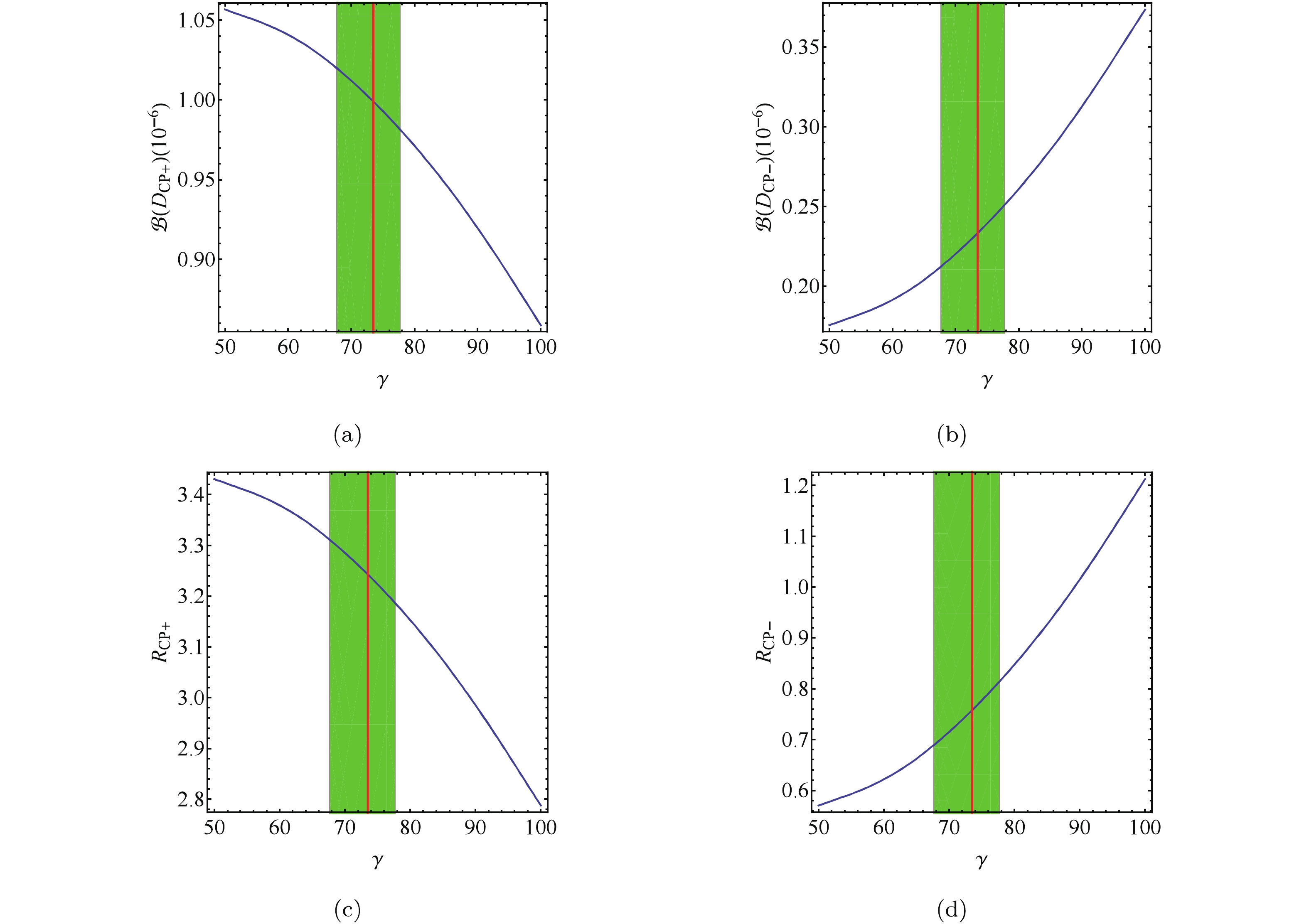
Figure 2. (color online) The dependence of the differential branching ratios
${\cal B}(\bar B_s^0 \to D_{{\rm CP}\pm}(\pi^+\pi^-)_S)$ on$\gamma$ are shown in panels (a,b). In panels (c,d), the corresponding physical observable that is measured$R_{{\rm CP}\pm}$ is shown as function of$\gamma$ . The shaded (green) regions denote the current bound$\gamma=73.5^{+4.2}_{-5.9}$ .${R_{{\rm CP} \pm }} = \frac{{4{\cal B}(\bar B_s^0 \to {D_{{\rm CP} \pm }}{{({\pi ^ + }{\pi ^ - })}_S})}}{{{\cal B}(\bar B_s^0 \to {D^0}{{({\pi ^ + }{\pi ^ - })}_S}) + {\cal B}(\bar B_s^0 \to {{\bar D}^0}{{({\pi ^ + }{\pi ^ - })}_S})}}.$

(35) The dependence of
$ R_{{\rm CP}\pm} $ on$ \gamma $ is shown in Fig. 2(c,d). The current bound for$ \gamma $ is$ \gamma = (73.5^{+4.2}_{-5.9})^\circ $ [63].The predicted dependence of the differential branching ratio
$ {\rm d}{\cal B}/{\rm d} m_{\pi\pi} $ on the pion-pair invariant mass$ m_{\pi\pi} $ is presented in Fig. 3(a) and Fig. 3(b) for the resonances$ f_0(500) $ ,$ f_0(980) $ ,$ f_0(1500) $ and$ f_0(1790) $ in the decays$ \bar B_s\to D^0 \pi^+\pi^- $ and$ \bar B_s\to \bar D^0 \pi^+\pi^- $ . The figures show that the main contribution to the two decays lies in the region around the pole mass$ m_{f_0(980)} = 0.97 $ , while$ f_0(500) $ gives a contribution primarily in the region below$ m_{\pi\pi} = 1~{\rm GeV} $ . The other resonances,$ f_0(1500) $ and$ f_0(1790) $ , still give considerable contributions to the processes. Therefore, we hope that more precise data from LHCb and the future KEKB may test our theoretical calculations.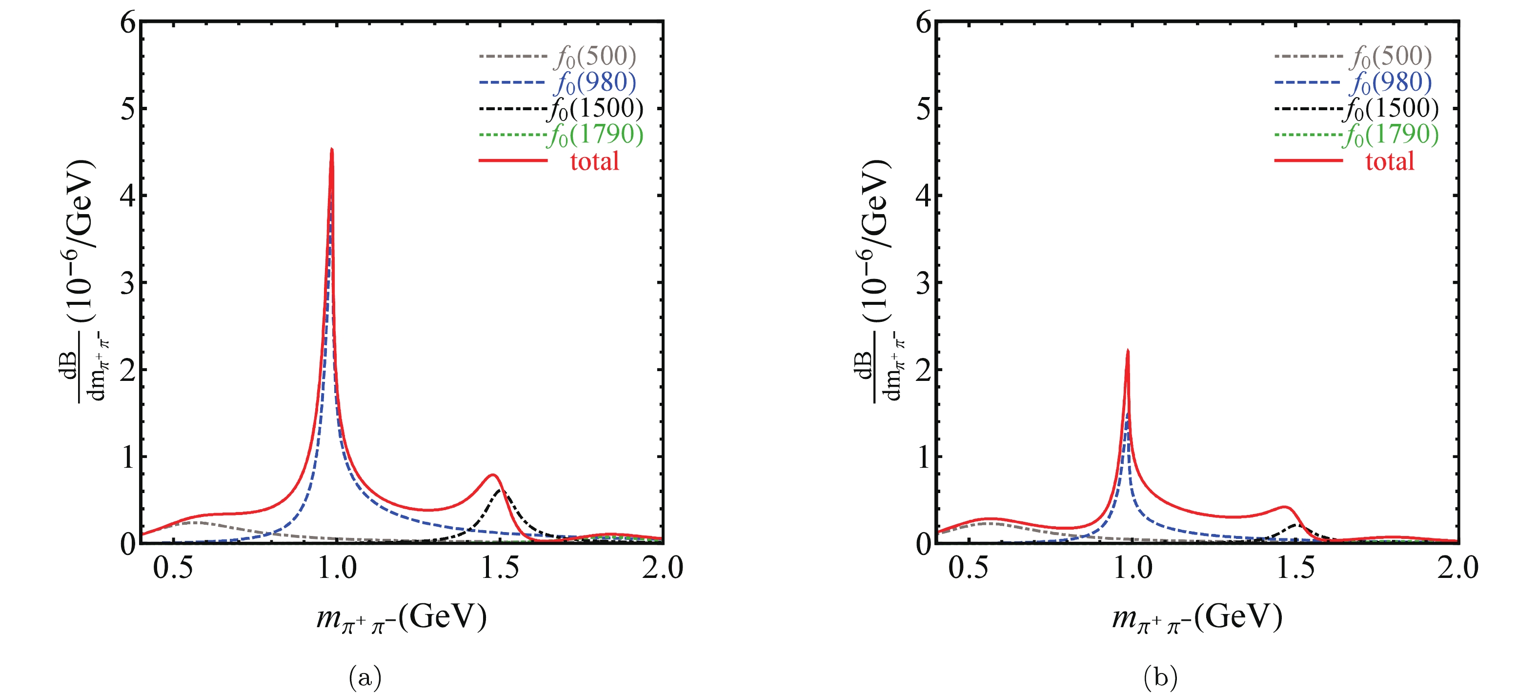
Figure 3. (color online) The dependence of the differential branching ratio on the pion-pair invariant mass for the resonances
$f_0(980)$ ,$f_0(1500)$ and$f_0(1790)$ in the decays (a)$\bar B_s^0\to D^0\pi^+\pi^-$ and (b)$\bar B_s^0\to \bar D^0\pi^+\pi^-$ . -
In the past decades, two-body B decays have provided an ideal platform for extracting the Standard Model parameters, and for probing new physics beyond SM [64, 65]. In this work, we studied the three-body decays
$ \bar B_s^0\to D^0(\bar D^0)\pi^+\pi^- $ within the PQCD framework, and in particular the S-wave contribution which was explicitly calculated. The S-wave two-pion light-cone distribution amplitudes can have both resonant$ f_0(500) $ ,$f_0(980), $ $ f_0(1500), f_0(1790) $ and nonresonant contributions. Furthermore, the processes proceed via tree level operators, and the branching ratios were found to be in the range from 10−7 to 10−6. It was found that the branching ratios are sensitive to the parameters$ \omega_b $ and$ a_2 $ in the$ B_s $ and two-pion distribution amplitudes. Therefore, we expect that future measurement could help to better understand the multi-body processes and the S-wave two-pion resonance and$ B_s $ distribution amplitudes.
S-wave contributions to ${{{\bar B}_s^0\to (D^0,{\bar D}^0)\pi^+\pi^-}}$ in the perturbative QCD framework
- Received Date: 2019-03-12
- Available Online: 2019-07-01
Abstract:


 DownLoad: