


 Abstract
 HTML
HTML Reference
 Related
 PDF
PDF


-
With only the loop diagram contributions in the Standard Model (SM), rare
$ B $ -mesons decays induced by flavor-changing neutral-current (FCNC) transitions provide an interesting possibility for exploring virtual effects from new physics (NP) beyond SM. Various FCNC processes, which are sensitive to any new source of flavor-violating interactions, are extensively studied in SM and in many of the extended models. With more and more precise experimental measurements, many NP parameters are severely constrained by these channels. Examples of this kind of decays are radiative, leptonic and semi-leptonic decays, which have relatively smaller theoretical hadronic uncertainties.Among the purely hadronic decays,
$ B\to K\pi $ decays have been studied in different NP scenarios [1,2]. In SM, the main contribution to these channels comes from the penguin-induced FCNC transition$ \bar b \to\bar s q \bar q $ $ (q = u,d) $ . Grossman et al. [3] studied the isospin-violating NP contributions in$ B\to K\pi $ decays. Focusing on$ B^\pm\to K\pi $ decays, these authors have explored the relevant observables for probing the parameter space of different NP models. In addition,$ B\to K\pi $ decays have been investigated as a solution of the so-called$ B\to K\pi $ puzzle in SM [4] and in different NP models [5,6]. However, from all these studies of rare hadronic decays, one can not make a definitive conclusion concerning new physics signals. One of the reasons is that the difficulties due to the theoretical hadronic uncertainties are much greater than expected.An alternative strategy is to search for rare
$ b $ decays, which have extremely small rates in SM, so that mere detection of such processes will indicate NP. Along these lines, Huitu et al. [7] have suggested the processes$ b\to ss\bar d $ and$ b\to dd\bar s $ as prototypes. In SM, the doubly weak transitions occur via box diagrams with up-type quarks and$ W $ inside loops, resulting in branching ratios of approximately$ {\cal{O}}(10^{-12}) $ and$ {\cal{O}}(10^{-14}) $ , respectively. Furthermore, both inclusive and exclusive channels for these transitions in different scenarios beyond SM have been investigated [8-13], and it is predicted that in different NP models they can be greatly enhanced. Notably, Pirjol and Zupan [14] performed a systematic study of two-body exclusive$ B\to PP,PV, VV $ modes based on$ b\to ss\bar d $ and$ b\to dd\bar s $ transitions, both in SM and for several NP models, such as NP with conserved global charge, minimal flavor violation (MFV), next-to-minimal flavor violation (NMFV) and general flavor violating models.However, the measurement of these two-body doubly weak decays, mediated by the
$ b\to dd\bar s $ and$ b\to ss\bar d $ transitions, is challenging, since in most cases they mix with the ordinary weak decays through$ B^0_{d,s}- $ $ \smash{\overline B}^0_{d,s} $ mixing or$ K^0- $ $ \smash{\overline K}^0 $ mixing. In the case of the$ b \to dd\bar s $ transition, the only suggested clear channels for experimental searches are the multi-body decays such as$ B^+\to \pi^+\pi^+K^- $ and$ B_s^0\to K^-K^-\pi^+\pi^+ $ , that occur either directly or via quasi two-body$ PV $ $ (B^+\to \pi^+\smash{\overline K}^{\ast0}) $ or$ VV $ $ (B_s^0\to \smash{\overline K}^{\ast0}\smash{\overline K}^{\ast0}) $ modes, respectively. Both B-factories have given the upper limit for the$ B^+\to \pi^+\pi^+K^- $ decay [15,16], whereas the latest one is reported by the LHCb collaboration to be$ {\cal{B}}(B^+\to \pi^+\pi^+K^-)<4.6\times 10^{-8} $ [17]. Due to the lack of reliable QCD predictions for branching ratios of three body decays, it is difficult to interpret these upper limits as constraints for the new physics parameters.In this paper, by employing the perturbative QCD factorization, we calculate the exclusive two-body pure annihilation decay
$ \smash{\overline B}^0\to K^+\pi^- $ induced by the$ b\to dd\bar s $ transition. This decay can occur only through the annihilation diagrams in SM because none of the quarks (antiquarks) in the final states are those of the initial$ B $ meson. It is extremely rare in SM. Therefore, any new physics contribution can be overwhelming. Since$ B^0 $ can mix with$ \smash{\overline B}^0 $ , it was thought previously that this channel is not distinguishable from the$ B^0\to K^+\pi^- $ decay with large branching ratio of the order of$ 10^{-5} $ . Here, we would like to point out that with a large data sample one can search for the suppressed wrong sign decay by performing a flavor-tagged time-dependent analysis, following Ref. [18]. Experimentally, one can identify$ B^0 $ or$ \smash{\overline B}^0 $ mesons at the production point, e.g. using the charge of the lepton from the semi-leptonic decay of the other$ B^0/\smash{\overline B}^0 $ meson. In general, the time-dependent decay rate of the initial$ \smash{\overline B}^0 (B^0) $ to the final state$ K^+\pi^- $ is proportional to$\exp(-\Gamma t)[1 \mp C \cos(\Delta mt) \pm $ $ S \sin(\Delta mt)] $ , where$ \Delta m $ and$ \Gamma $ are the mass difference and decay width of the$ B^0- $ $ \smash{\overline B}^0 $ system. Without the wrong sign decay, one expects$ C = 1 $ and$ S = 0 $ . This can be tested at Belle-II, LHCb and its future upgrade. Any deviation from$ C = 1 $ and$ S = 0 $ is a signal of the wrong sign$ \smash{\overline B}^0\to K^+\pi^- $ decay, which may give an indication of new physics.In this work, we also found another advantage of the wrong sign
$ \smash{\overline B}^0\to K^+\pi^- $ decay. The effective operators involved in the doubly weak decays$ b\to dd\bar s $ and$ b\to ss\bar d $ , usually also contribute to$ K^0- $ $ \smash{\overline K}^0 $ and$ B^0- $ $ \smash{\overline B}^0 $ mixing, or$ B_s^0- $ $ \smash{\overline B}_s^0 $ mixing. Thus they are severely constrained by the mixing parameters measured in high precision experiments, which cannot contribute much to the hadronic$ B $ decays. On the contrary, in a particular NP model with conserved charge, some of the new physics operators that contribute to the wrong sign$ \smash{\overline B}^0\to K^+\pi^- $ decay through the annihilation diagram may not be severely constrained by the meson mixing parameters, due to the hierarchies among the NP couplings. These operators, with pseudoscalar density structure, survive helicity suppression by the chiral enhancement mechanism. This can lead to a branching ratio of the wrong sign decay which is sufficiently large to be measured by experiments. Even in the absence of the signal, with only an upper limit, the measurements of this type of decay will at least give the most stringent constraint on the new physics parameters.The paper is organized as follows. In Sec. 2, we calculate the decay rate for the chosen process in SM. In Sec. 3, we consider a model independent analysis of the considered channel and give predictions for NP contributions in different NP scenarios. Next, we consider how a specific NP model with tree level FCNC transitions, such as the Randall-Sundrum (RS) model [19,20], could enhance the decay rate of
$ \smash{\overline B}^0\to K^+\pi^- $ , while satisfying all relevant constraints. For this study, we consider two models known as the RS model with custodial protection$ ({\rm {RS}}_c) $ [21-25] in Sec. 4, followed by the bulk-Higgs RS model [26] in Sec. 5. Relevant bounds and numerical results for the two variants of the RS model are given in Sec. 6. Lastly, we summarize our results in Sec. 7. -
The doubly weak decay
$ b \to dd\bar s $ can only occur in SM through the box diagram, which is highly suppressed. The local effective Hamiltonian for the$ b \to dd\bar s $ transition is given by$ {\cal{H}}^{\rm{SM}} = C^{\rm{SM}}[(\bar d_L^{\alpha}\gamma^{\mu}b_L^{\alpha})(\bar d_L^{\beta}\gamma_{\mu}s_L^{\beta})], $

(1) where
$ C^{\rm{SM}} = \frac{G_F^2m_W^2}{4\pi^2}V_{tb}V_{td}^*\left[V_{ts}V_{td}^*f (x)+V_{cs}V_{cd}^*\frac{m_c^2}{m_W^2}g(x,y)\right], $

(2) with functions
$ f(x) $ and$ g(x,y) $ given explicitly in [7], where$ x = m_W^2/m_t^2 $ ,$ y = m_c^2/m_W^2 $ .The exclusive
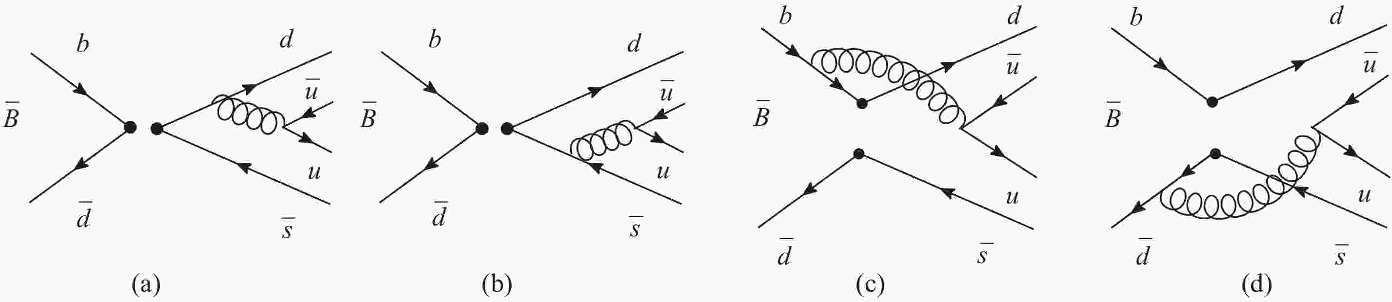
$ \smash{\overline B}^0\to K^+\pi^- $ decay, induced by the$ b \to dd\bar s $ transition, can only occur through the annihilation type Feynman diagrams. In the perturbative QCD framework (PQCD), according to the effective Hamiltonian, the four lowest order annihilation Feynman diagrams for$ \smash{\overline B}^0\to K^+\pi^- $ decay are shown in Fig. 1, where ($ a $ ) and ($ b $ ) are factorizable diagrams, while ($ c $ ) and ($ d $ ) are nonfactorizable. The initial$ b $ and$ \bar d $ quarks annihilate into$ d $ and$ \bar s $ quarks, which then form a pair of light mesons by hadronizing with another pair of$ u\bar u $ produced perturbatively through the one gluon exchange mechanism.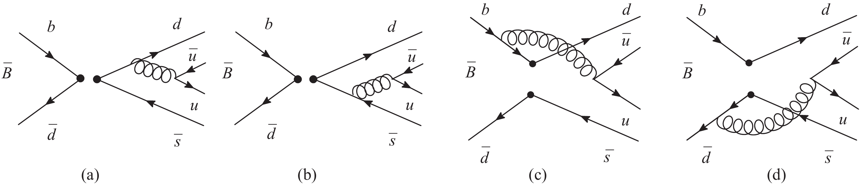
Figure 1. Feynman diagrams which contribute to the
$ \smash{\overline B}^0\to K^+\pi^- $ decay to leading order, ($ a $ ) and ($ b $ ) are factorizable diagrams, ($ c $ ) and ($ d $ ) are nonfactorizable.We consider
$ \smash{\overline B}^0 $ meson at rest for simplicity. It is convenient to use light-cone coordinates ($ P^+, P^-, { k}_T $ ), which are defined as:$ \begin{align} P^+ = \frac{p_0+p_3}{\sqrt 2},\,\, P^- = \frac{p_0-p_3}{\sqrt 2},\,\,{ k}_T = (p_1,p_2). \end{align} $

(3) The
$ \smash{\overline B}^0 $ meson momentum$ P_1 $ and the momenta of$ K^+ $ and$ \pi^- $ meson, denoted respectively by$ P_2 $ and$ P_3 $ , can be written as$ \begin{align} P_1 = \frac{m_B}{\sqrt 2}(1,1,{\bf 0}_T),\quad P_2 = \frac{m_B}{\sqrt 2}(1,0,{\bf 0}_T),\quad P_3 = \frac{m_B}{\sqrt 2}(0,1,{\bf 0}_T). \end{align} $

(4) The antiquark momenta
$ k_1 $ ,$ k_2 $ and$ k_3 $ in$ \smash{\overline B}^0 $ ,$ K^+ $ and$ \pi^- $ meson are taken as$ \begin{align} k_1 = (0,x_1P_1^{-},{ k}_{1T}), \; k_2 = (x_2P_2^{+},0,{ k}_{2T}), \; k_3 = (0,x_3P_3^{-},{ k}_{3T}), \end{align} $

(5) where the light meson masses have been neglected. In PQCD [27-31], the decay amplitude is factorized into soft (
$ \Phi $ ), hard ($ H $ ) and harder ($ C $ ) dynamics characterized by different scales$ \begin{aligned} {\cal{A}}&\sim\int {\rm d}x_1 {\rm d}x_2 {\rm d}x_3 b_1 {\rm d}b_1 b_2 {\rm d}b_2 b_3 {\rm d}b_3 \\&\times {\rm{Tr}}\Big[C(t)\Phi_B(x_1,b_1) \otimes\Phi_{K }(x_2,b_2)\otimes\Phi_{\pi}(x_3,b_3)\\&\times \left. H(x_i,b_i,t)S_t(x_i)e^{-S(t)}\right], \end{aligned} $

(6) where Tr denotes the trace over Dirac and color indices, and
$ b_i $ are conjugate variables to$ { k}_{i T} $ of the valence quarks. The universal wave function$ \Phi_M(x_i,b_i) $ ($ M = B,K,\pi $ ), describing hadronization of the quark and anti-quark into a meson$ M $ , can be determined in other decays. The explicit formulas are given in Appendix A. The factorization scale$ t $ is the largest energy scale in$ H $ , as a function of$ x_i $ and$ b_i $ . The Wilson coefficient$ C(t) $ results from the radiative corrections at short distances, which includes the harder dynamics at a scale larger than the$ m_B $ scale, and describes the evolution of the local 4-Fermi operators from$ m_W $ down to the$ t $ scale. Using the threshold resummation [32], the large doubly logarithms ($ \ln^2x_i $ ) are summed, leading to$ S_t(x_i) $ which suppresses the end-point contributions.$ e^{-S(t)} $ , called the Sudakov form factor [33], contains resummation of two kinds of logarithms. One of the large logarithms is due to the renormalization of the ultra-violet divergence$ \ln tb $ , and the other is a doubly logarithm$ \ln^2b $ arising from the overlap of collinear and soft gluon corrections. Such factors suppress effectively the soft dynamics, making the perturbative calculation of the hard part$ H $ reliable.By inserting the SM operator given in Eq. (1) into the vertices of each Feynman diagram, we calculate the hard part
$ H $ to first order in$ \alpha_s $ and obtain the analytic formulas$ F_{a1} $ and$ {\cal M}_{a1} $ , which represent the factorizable and nonfactorizable annihilation diagram contributions, respectively. The explicit expressions for$ F_{a1} $ and$ {\cal M}_{a1} $ are given in Appendix B. It is obvious that these annihilation type contributions are suppressed compared to the emission diagrams, which agrees with the helicity suppression argument. Finally, the total amplitude for the considered process in SM is given as$ \begin{aligned} {\cal{A}}^{\rm{SM}} = F_{a1}\bigg[\frac{4}{3}C^{\rm{SM}}\bigg]+{\cal{M}}_{a1}\bigg[C^{\rm{SM}}\bigg], \end{aligned} $

(7) with the expression for the decay rate
$ \begin{aligned} \Gamma^{\rm{SM}} = \frac{m_{B}^3}{64\pi}\left|{\cal{A}}^{\rm{SM}}\right|^2, \end{aligned} $

(8) we calculate the branching fraction of the
$ \smash{\overline B}^0\to K^+\pi^- $ decay in SM$ \begin{aligned} {\cal{B}}(\smash{\overline B}^0\to K^+\pi^-)^{\rm{SM}} = 1.0\times 10^{-19}. \end{aligned} $

(9) Obviously, this is well below the current experimental measurement abilities, so this channel can turn out to be an ideal probe of NP effects.
-
In this section we present a model independent analysis of the NP contributions to the exclusive decay
$ \smash{\overline B}^0\to K^+\pi^- $ . We start with the most general local effective Hamiltonian with all possible dimension-6 operators [3]$ \begin{align} {\cal{H}}_{\rm{eff}}^{\rm{NP}} = \sum_{j = 1}^5[C_j{\cal{O}}_j+\widetilde {C}_j\widetilde{\cal{O}}_j], \end{align} $

(10) where
$ \begin{split} &{\cal{O}}_1 = (\bar d_L\gamma_{\mu} b_L)(\bar d_L\gamma^{\mu} s_L),\\ &{\cal{O}}_2 = (\bar d_R b_L)(\bar d_R s_L),\,\,\,\,\,\, {\cal{O}}_3 = (\bar d_R^{\alpha} b_L^{\beta})(\bar d_R^{\beta}s_L^{\alpha}),\\ &{\cal{O}}_4 = (\bar d_R b_L)(\bar d_L s_R),\,\,\,\,\,\, {\cal{O}}_5 = (\bar d_R^{\alpha} b_L^{\beta})(\bar d_L^{\beta}s_R^{\alpha}). \end{split} $

(11) The
$ \widetilde O_j $ operators represent the chirality flipped operators which can be obtained from$ O_j $ by$ L\leftrightarrow R $ exchange. In SM, only$ {\cal{O}}_1 $ is present. The new physics beyond SM can change the Wilson coefficient of operator$ O_1 $ , and it can also provide non zero Wilson coefficients for the other operators. These Wilson coefficients are not free parameters, as all of them also contribute to$ K^0-\smash{\overline K}^0 $ and$ B^0-\smash{\overline B}^0 $ mixing. The experimentally well measured mixing parameters give stringent constraints on the Wilson coefficients. This is the main reason why in many new physics models one can not get large branching ratios for the$ b\to dd \bar s $ or$ b\to ss \bar d $ decays, see for example [34].We first assume that NP only gives a contribution to the local operator
$ {\cal{O}}_1 $ similar to SM, which is true for a large class of NP models including the two-Higgs doublet model (2HDM) with small tan$ \beta $ , or the constrained minimal supersymmetry standard model (MSSM) [13]. The NP Hamiltonian for the$ b \to dd\bar s $ transition in this case is the same as for SM in Eq. (1), but with a new Wilson coefficient$ C_{1}^{dd\bar s} $ . The decay width of$ \smash{\overline B}^0\to K^+\pi^- $ will also have the same formula as in the SM case. The corresponding Hamiltonians for$ K^0-\smash{\overline K}^0 $ and$ B^0-\smash{\overline B}^0 $ mixing are$ \begin{align} [{\cal{H}}_{\rm{eff}}^{\Delta S = 2}] = C_{1}^{K}(\bar d_L\gamma_{\mu} s_L)(\bar d_L\gamma^{\mu} s_L), \end{align} $

(12) $ \begin{align} [{\cal{H}}_{\rm{eff}}^{\Delta B = 2}] = C_{1}^{B_d}(\bar d_L\gamma_{\mu} b_L)(\bar d_L\gamma^{\mu} b_L), \end{align} $

(13) where the coefficients in general have the form
$ C_{1}^{dd\bar s}\sim \sqrt{C_{1}^{K} C_{1}^{B_d}} $ . Since the SM results for$ K^0\text{-}\smash{\overline K}^0 $ and$ B^0\text{-}\smash{\overline B}^0 $ mixing are in good agreement with the experimental data, there is not much room left for the new physics contributions.Next, if the NP contributions come from the non-standard model chiralities, and considering each non-standard operator in
$ {\cal{O}}_{j} $ individually, the decay amplitude is given by$ \begin{aligned} {\cal{A}}_j(\smash{\overline B}^0\to K^+\pi^-) = F_{aj}\bigg[\frac{4}{3}C_j^{dd \bar s}\bigg]+{\cal{M}}_{aj}\bigg[C_j^{dd\bar s}\bigg], \end{aligned} $

(14) where
$ j = 2,3,4, 5 $ . The explicit expressions for$ F_{a2,a3,a4,a5} $ and$ {\cal M}_{a2,a3,a4,a5} $ are given in Appendix B. Similarly, for$ \widetilde{\cal{O}}_{1-5} $ , we have$ \begin{aligned} \widetilde{\cal{A}}_j(\smash{\overline B}^0\to K^+\pi^-) = F_{aj}\bigg[\frac{4}{3}\widetilde{C}_j^{dd \bar s}\bigg]+{\cal{M}}_{aj}\bigg[-\widetilde{C}_j^{dd\bar s}\bigg]. \end{aligned} $

(15) The corresponding decay widths of each individual operator
$ {\cal{O}}_{2-5} $ and$ \widetilde{\cal{O}}_{1-5} $ are given by$ \begin{aligned} \Gamma_j(\smash{\overline B}^0\to K^+\pi^-) = \frac{m_{B}^3}{64\pi}\left|{\cal{A}}_j(\smash{\overline B}^0\to K^+\pi^-)\right|^2, \end{aligned} $

(16) $ \begin{aligned} \widetilde{\Gamma}_j(\smash{\overline B}^0\to K^+\pi^-) = \frac{m_{B}^3}{64\pi}\left|\widetilde{\cal{A}}_j(\smash{\overline B}^0\to K^+\pi^-)\right|^2, \end{aligned} $

(17) We define the ratio
$ R $ of the branching ratio of the wrong sign decay to the corresponding SM branching ratio of the right sign decay (induced by the$ b \to su\bar u $ ),$ \begin{aligned} R\equiv \frac{{\cal{B}}(\smash{\overline B}^0\to K^+\pi^-)}{{\cal{B}}(\smash{\overline B}^0\to K^-\pi^+)}. \end{aligned} $

(18) We consider the corresponding LO PQCD prediction for the right sign decay, whose amplitude is given by Eq. (22) of [28], while the numerical predictions of the factorizable and nonfactorizable amplitudes are listed in Table 1 of [28]. With a direct experimental measurement of the ratio
$ R $ , one can give a constraint for each individual Wilson coefficient of the new physics operator in Eq. (11). As an example, by considering each non-standard model NP operator, we give in Table 1 the upper bound on the corresponding Wilson coefficient by assuming that the current experimental precision can limit the ratio$ R $ to less than$ 0.001 $ .parameter allowed range/ (GeV−2) $ \widetilde C_1 $ 

$<1.1\times 10^{-7} $ 

$ C_2 $ 

$<6.3\times 10^{-9} $ 

$ \widetilde C_2 $ 

$<6.8\times 10^{-9} $ 

$ C_3 $ 

$<5.1\times 10^{-8} $ 

$ \widetilde C_3 $ 

$<5.3\times 10^{-8} $ 

$ C_4 $ 

$<4.9\times 10^{-9} $ 

$ \widetilde C_4 $ 

$<4.2\times 10^{-9} $ 

$ C_5 $ 

$<1.6\times 10^{-6} $ 

$ \widetilde C_5 $ 

$<7.3\times 10^{-7} $ 

Table 1. Upper bounds on the Wilson coefficients of the non-standard new physics operators obtained by assuming an experimental precision of
$ R<0.001 $ . -
We start with an NP scenario that involves the exchange of NP fields carrying a conserved charge. A particular example of a scenario of this type is the
$ R$ -parity violating MSSM [13]. In this class, one can start with NP Lagrangian of a generic form [14]$ \begin{split} {\cal{L}}_{\rm{flavor}} =& g_{b\to d}(\bar d \Gamma b)X+g_{d\to b}(\bar b \Gamma d)X+g_{s\to d}(\bar d \Gamma s)X\\&+g_{d\to s}(\bar s \Gamma d)X+\rm{h.c.}, \end{split} $

(19) assuming that field
$ X $ with mass$ M_X $ carries a conserved quantum number broken only by the above terms. Flavor changing operators are then obtained after integrating out field$ X $ . In this example, one can consider the hierarchies in NP couplings such that the mixing constraints can be trivially satisfied, leaving the$ b \to dd\bar s $ transitions unbounded. To illustrate this point, we consider four scenarios. In scenario 1 (S1) and scenario 2 (S2), we consider that NP matches onto the local operators$ {\cal{O}}_1 $ and$ \cal{\widetilde{O}} $ 1, respectively, while in scenario 3 (S3) and scenario 4 (S4), NP matches onto the linear combination of local operators$ {\cal{O}}_4 $ ,$ \cal{\widetilde{O}} $ 4 and$ {\cal{O}}_5 $ ,$ \cal{\widetilde{O}} $ 5, respectively. As S2, S3 and S4 involve local operators with non-standard chiralities, it will be convenient to define the normalized matrix elements of these non-standard operators with respect to the SM operator$ {\cal{O}}_1 $ .$ \begin{aligned} r_j(B\to M_2 M_3)\equiv \frac{\langle M_2M_3 |{\cal{O}}_j| B\rangle}{\langle M_2M_3 |{\cal{O}}_1| B\rangle}, \end{aligned} $

(20) where
$ j = 2,3,4,5 $ . Similarly for$ \cal{\widetilde{O}} $ 1-5, where we denote the ratio as$ {\widetilde r}_j $ .Starting with S1 and S2, the NP Hamiltonians are given by
$ [{\cal{H}}_{\rm{S1}}^{dd\bar s}] = C_1^{dd\bar s}\eta_{\rm{QCD}}{\cal{O}}_1 $ ,$[{\cal{H}}_{\rm{S2}}^{dd\bar s}] = $ $ {\widetilde C}_1^{dd\bar s}\eta_{\rm{QCD}}\cal{\widetilde {O}} $ 1, where$ C_1^{dd\bar s}\!\! =\!\! {\widetilde C}_1^{dd\bar s}\!\! =\!\!\displaystyle\frac{1}{M_{X}^2}\big(g_{b\to d}g_{d\to s}^{\ast}\!+\! g_{s\to d}g_{d\to b}^{\ast}\big) $ . As for the RG running of the coefficients$ C_1^{dd\bar s} $ and$ {\widetilde C}_1^{dd\bar s} $ from the weak scale$ m_W $ to$ m_b $ , we suppose that there is no new particle within these scales, and that the evolution of both coefficients is the same as in QCD. The evolution factor to NLO is given by$ \eta_{\rm{QCD}}(m_b) = 0.87 $ . For S3 and S4, the NP Hamiltonians and the corresponding Wilson coefficients can be written as$[{\cal{H}}_{\rm{NP}}^{dd\bar s}] = f_{j\rm{QCD}}\Big({C_j^{dd\bar s}{\cal{O}}_j}+$ $ {\widetilde C}_j^{dd\bar s}{\cal{\widetilde {O}}}_j\Big) $ and$ C_j^{dd\bar s} = $ $ 1/{M_{X}^2}(g_{b\to d}g_{d\to s}^{\ast}) $ ,${\widetilde C}_j^{dd\bar s} = {1}/{M_{X}^2} $ $ (g_{s\to d}g_{d\to b}^{\ast}) $ , with$ j = 4, 5 $ for S3 and S4, respectively. Similarly to the previous case, we factor out NLO QCD corrections for the Wilson coefficients in S3 and S4. However, the situation is different here as the operators$ {\cal{O}}_4(\cal{\widetilde {O}}) $ 4 and$ {\cal{O}}_5(\cal{\widetilde {O}}) $ 5 mix under renormalization such that the RG evolution operator is a$ 2\times2 $ matrix, so that each Wilson coefficient gets a small mixing induced contribution at NLO, which we ignore. Therefore, keeping only the dominant contributions we obtain$ f_{4\rm{QCD}} = 2 $ , while$ f_{5\rm{QCD}} = 0.9 $ . Considering the corresponding Hamiltonians in all four scenarios, we get the bounds for$ K^0-\smash{\overline K}^0 $ and$ B^0-\smash{\overline B}^0 $ mixing$ \begin{aligned} \frac{|g_{s\to d}g_{d\to s}^{\ast}|}{M_{X}^2}<\frac{1}{(\Lambda_j^K)^2},\qquad\;\:\frac{|g_{b\to d}g_{d\to b}^{\ast}|}{M_{X}^2}<\frac{1}{(\Lambda_j^{B_d})^2}, \end{aligned} $

(21) where
$ j = 1 $ for S1 and S2, while S3 and S4 correspond to$ j = 4, 5 $ , respectively. Considering the relations$ |C_{j}^{v}| = 1/(\Lambda_j^v)^2 $ ,$ |{\widetilde C}_{1}^{v}| = 1/(\Lambda_1^v)^2 $ , where$ v = K, B_d $ , for$ K^0\text{-}\smash{\overline K}^0 $ and$ B^0\text{-}\smash{\overline B}^0 $ mixing, respectively, the lower bounds on the NP scales$ \Lambda_j^K $ and$ \Lambda_j^{B_d} $ [35] are listed in Table 2, with Im$ (C_j^K) $ additionally constrained from$ \epsilon_K $ .operators $K^0-\smash{\overline K}^0$ 

$B^0-\smash{\overline B}^0$ 

parameter lower limit/TeV parameter lower limit/TeV ${\cal{O}}_1$ 

$\Lambda_1^K$ 

$1\times 10^3$ 

$\Lambda_1^{B_d}$ 

210 ${\cal{O}}_2$ 

$\Lambda_2^K$ 

$7.3\times 10^3$ 

$\Lambda_2^{B_d}$ 

$1.2\times 10^3$ 

${\cal{O}}_3$ 

$\Lambda_3^K$ 

$4.1\times 10^3$ 

$\Lambda_3^{B_d}$ 

600 ${\cal{O}}_4$ 

$\Lambda_4^K$ 

$17\times 10^3$ 

$\Lambda_4^{B_d}$ 

$2.2\times 10^3$ 

${\cal{O}}_5$ 

$\Lambda_5^K$ 

$10\times 10^3$ 

$\Lambda_5^{B_d}$ 

$1.3\times 10^3$ 

Table 2. Lower bounds on the NP scales coming from
$K^0-\smash{\overline K}^0$ and$B^0-\smash{\overline B}^0$ mixing [35].To keep the
$ b \to dd\bar s $ transition unbounded and large, we take as case-I$ g_{d\to s} = g_{b\to d} = 1 $ , where the bounds in (21) can be trivially satisfied, if for instance$ g_{s\to d} = g_{d\to b} = 0 $ . As mixing bounds do not constrain$ M_{X} $ in this case, the ratio$ R_X $ can be as large as possible. For example, after assuming that the NP scale$ M_{X} $ lies around the TeV scale, the obtained ratio$ R_X $ in each scenario is listed under case-I in Table 3. One can see that the resulting ratio$ R_X $ , after satisfying the mixing constraints, is very large in each scenario compared to the SM result ($ R_{\rm{SM}} $ ). Therefore, the measurement of the ratio$ R_X $ , with an upper limit for the$ \smash{\overline B}^0\to K^+\pi^- $ branching ratio if no signal is found, will provide the most stringent constraint on the operators in this example of NP.scenarios $ R_X $ 

$ R_{\rm{SM}} $ 

$ M_X $ /TeV

case-I $ M_X $ /TeV

case-II S1 1.0 0.085 10 $ 8.5\times 10^{-6} $ 

$ 6.8\times 10^{-15} $ 

S2 0.074 $ 7.3\times 10^{-6} $ 

S3 55 $ 0.005 $ 

S4 0.002 $ 1.9\times 10^{-7} $ 

Table 3. Ratio of the branching fraction for the wrong sign decay to the branching fraction for the right sign decay, after satisfying the mixing constraints, in the case of NP involving conserved charge
$ (R_X) $ .$ \rm{S}1-\rm{S}4 $ represent NP scenarios corresponding to the presence of different NP operators (see text for details).Further, we assume a higher NP scale at
$ 10 $ TeV. The resulting PQCD prediction for the ratio$ R_X $ in corresponding scenarios is listed in Table 3 as case-II. In scenario S3, the predicted ratio, after satisfying the mixing constraints, is large enough to provide stringent constraint for the coefficient of the operators$ {\cal{O}}_4 $ or$ \cal{\widetilde{O}} $ 4. On the other hand, the obtained ratio$ R_X $ in (S1, S2) and S4 give nine and eight orders of magnitude increase, respectively, compared to the SM result, although it is very difficult to reach such a precision experimentally.As case-III, we consider the situation where accidentally one of the
$ g_i $ couplings is very small. For example, if we take$ g_{s\to d} = 0 $ and all the other$ g_i = 1 $ , then$ K^0-\smash{\overline K}^0 $ mixing bounds in (21) are trivially satisfied, while$ B^0-\smash{\overline B}^0 $ mixing yields a lower bound on$ M_{X} $ . In this case, the bound on$ M_{X} $ is in each scenario more stringent compared to the previous cases. Therefore, the predictions for the ratio$ R $ obtained for scenarios S1, S2, S3 and S4 are of the order of$ 10^{-11} $ ,$ 10^{-12} $ and$ 10^{-16} $ , respectively. However, compared to$ R_{\rm{SM}} $ , as given in Table 3, S1 and S2 give four and three orders of magnitude enhancement, respectively. -
In MFV [36], the coefficients can be considered as
$ C_j^v = \displaystyle\frac{F_j^v}{[{(\Lambda_{\rm{MFV}})}_{_j}^{v}]^2} $ , where$ v = dd\bar s, K, B_d $ for the$ b \to dd\bar s $ transition, and$ K^0-\smash{\overline K}^0 $ and$ B^0-\smash{\overline B}^0 $ mixing, respectively. First, we consider the class of MFV models in which$ \Delta F = 2 $ processes are strongly dominated by the same single operator with the$ (V-A)\times (V-A) $ structure [36], as in the low energy effective Hamiltonian of SM. All the other non-standard operators ($ {\cal{O}}_{2-5} $ and$ \widetilde{\cal{O}}_{1-5} $ ), if generated, are suppressed and do not contribute significantly. For instance, in the MFV effective theory [36], the non-standard dimension-6 FCNC operators for$ \Delta F = 2 $ processes involving external down-type quarks can be constructed with the bilinear FCNC structure of the form$ \bar D_R \lambda_d \lambda_{\rm{FC}} Q_L $ , where$ \lambda_{\rm{FC}} $ represents the effective coupling for all FCNC processes with external down-type quarks. Therefore, the constructed operators will be suppressed by the Yukawa couplings ($ \lambda_{d_i} $ ) corresponding to the external masses. Example of this class of models are 2HDM II and MSSM, provided that$ \tan \beta $ (the ratio between the two vacuum expectation values of the two-Higgs doublet) is not too large. Therefore, in the MFV case with small/moderately large$ \tan \beta $ , we have$ F_1^v = F_{\rm{SM}}^v $ and$ F_{j\neq1}^v = 0 $ .$ F_{\rm{SM}}^v $ are the appropriate CKM matrix elements, such as$ F_{\rm{SM}}^{dd\bar s} = V_{tb}V_{td}^*V_{ts}V_{td}^* $ ,$ F_{\rm{SM}}^{K} = (V_{ts}V_{td}^*)^2 $ and$ F_{\rm{SM}}^{B_d} = (V_{tb}V_{td}^*)^2 $ . In this case, the UTfit collaboration has given, from a global fit, a model independent lower bound on the MFV scale$ {(\Lambda_{\rm{MFV}})}_{_1} $ at 95% probability, such that$ {(\Lambda_{\rm{MFV}})}_{_1}>5.5\;(5.1) $ TeV for small (moderately large)$ \tan \beta $ [35]. We define the suppression scales that include the hierarchy of the NP induced flavor changing couplings, such that$ \begin{split} \frac{F_{\rm{SM}}^{dd\bar s}}{[{(\Lambda_{\rm{MFV}})}_{_1}^{dd\bar s}]^2}\equiv &\frac{1}{(\Lambda_1^{dd\bar s})^2},\qquad \; \frac{F_{\rm{SM}}^{K}}{[{(\Lambda_{\rm{MFV}})}_{_1}^{K}]^2}\equiv\frac{1}{(\Lambda_1^{K})^2},\\ &\frac{F_{\rm{SM}}^{B_d}}{[{(\Lambda_{\rm{MFV}})}_{_1}^{B_d}]^2}\equiv\frac{1}{(\Lambda_1^{B_d})^2}. \end{split} $

(22) With all parameters known, one observes that the suppression scale
$ \Lambda_1^{dd\bar s} $ is the geometric average of the NP scales in$ K^0-\smash{\overline K}^0 $ and$ B^0-\smash{\overline B}^0 $ mixing,$ \Lambda_1^{dd\bar s} = \sqrt {\Lambda_1^K \Lambda_1^{B_d}} $ . The resulting order of magnitude prediction for the ratio$ R({\cal{O}}_1) $ is$ 10^{-16} $ for small$ \tan \beta $ , while it is of the same order as the SM prediction for moderately large$ \tan \beta $ .Next, we consider the class of MFV models, often called generalized MFV models (GMFV), in which the non-standard operators (
$ {\cal{O}}_{2-5} $ and$ \widetilde{\cal{O}}_{1-5} $ ) are allowed to contribute significantly to the$ \Delta F = 2 $ processes. The above mentioned models, 2HDM II and MSSM, transform to GMFV models for very large$ \tan \beta $ [37]. Generally, in models with a two-Higgs doublet and very large$ \tan \beta $ , the most prominent contributions from the non-standard operators to the$ \Delta F = 2 $ processes with external down-type quarks, come from the$ {\cal{O}}_{4} $ operator, which originates in the MFV effective theory as$ (\bar D_R \lambda_d \lambda_{\rm{FC}} Q_L) $ $(\bar Q_L \lambda_{\rm{FC}} \lambda_d D_R) $ [36]. Although still suppressed by the Yukawa couplings ($ \lambda_{d_i} $ ), the corresponding$ {\cal{O}}_{4} $ operators in the case of$ B_q^0-\smash{\overline B}_q^0 $ mixing ($ q = d, s $ ), give non-negligible contributions for very large$ \tan \beta $ , so that [36]$ \begin{align} C_4^{B_q} = \frac{(a_0+a_1)(a_0+a_2)}{[{(\Lambda_{\rm{MFV}})}_{_4}^{B_q}]^2}\lambda_b \lambda_q F_{\rm{SM}}^{B_q}. \end{align} $

(23) In this case, the UTfit collaboration obtained the lower bound on
$ {(\Lambda_{\rm{MFV}})}_{_4} $ , which represents the NP scale corresponding to the mass of non-standard Higgs bosons [35]$ \begin{align} {(\Lambda_{\rm{MFV}})}_{_4}\equiv M_H > 5 \sqrt{(a_0+a_1)(a_0+a_2)}\left(\frac{\tan \beta}{50}\right) \rm{TeV}. \end{align} $

(24) In order to give a prediction for the ratios
$ R({\cal{O}}_4) $ and$ R(\cal{\widetilde{O}} $ 4), it is required to opt for a specific model to obtain the$ a_{0,1,2} $ factors, which represent the$ \tan \beta $ -enhanced loop factors of$ \cal{O} $ (1). However, irrespective of the particular values of$ a_{0,1,2} $ and$ \tan \beta $ , the prediction of$ R({\cal{O}}_4) $ and$ R(\cal{\widetilde{O}} $ 4) will be smaller than$ R_{\rm{SM}} $ because of the suppressed Yukawa couplings in$ C_4^{dd\bar s} $ and$ {\widetilde C}_4^{dd\bar s} $ .In NMFV [38], we have
$ |F_j^v| = F_{\rm{SM}}^v $ with an arbitrary phase, so that the strict correlation between the Wilson coefficients is lost, and we have approximately$ \Lambda_j^{dd\bar s}\sim \sqrt {\Lambda_j^K \Lambda_j^{B_d}} $ . Considering each operator$ {\cal{O}}_j $ separately, one can obtain the approximate value of the suppression scale$ \Lambda_j^{dd\bar s} $ by using the bounds from Table 2. The corresponding PQCD predictions for the ratio$ R({\cal{O}}_j) $ , with$ j = 1,2,3,4,5 $ , are of$ {\cal{O}}(10^{-12}) $ ,$ {\cal{O}}(10^{-13}) $ ,$ {\cal{O}}(10^{-14}) $ ,$ {\cal{O}}(10^{-14}) $ and$ {\cal{O}}(10^{-17}) $ , respectively. Although the PQCD amplitudes for the$ {\cal{\widetilde{O}}}_{j} $ operators are slightly different, the predictions of the order of magnitude for the ratios$ R({\cal{\widetilde{O}}}_{j}) $ remain the same.The model-independent results of the UTfit group [35] suggested that the scale of heavy particles mediating tree-level FCNC in NMFV models must be heavier than
$ \sim 60 $ TeV. An application of these results to the RS-type models [39] showed that the measured value of$ \epsilon_K $ implies that the mass scale of the lightest KK gluon must lie above$ \sim 21 $ TeV, if the hierarchy of the fermion masses and weak mixings is solely due to the geometry, and the 5D Yukawa couplings are anarchic and of$ \cal{O} $ (1). A follow up study of the$ {\rm{RS}}_c $ model [40], while confirming the results of [39], pointed out that there exist regions in parameter space, without much fine-tuning of the 5D Yukawa couplings, which satisfy all$ \Delta F = 2 $ and EW precision constraints for the masses of the lightest KK gauge bosons,$ M_{\rm{KK}}\simeq3 $ TeV. Therefore, in a specific NMFV model the bounds, including the accidental cancellations of the contributions of different operators, can be weaker. We study the$ \smash{\overline B}^0\to K^+\pi^- $ decay in the RS-type models below. Moreover, while considering any specific NP model one must consider additional bounds, apart from those from$ K^0-\smash{\overline K}^0 $ and$ B^0-\smash{\overline B}^0 $ mixing.Finally, we assume that the NP scale is at the mass scale probed by
$ K^0-\smash{\overline K}^0 $ mixing, such that the corresponding$ \Lambda_j^K $ are given in Table 2, and all flavor violating couplings are of$ {\cal{O}}(1) $ . The resulting ratio$ R({\cal{O}}_1) $ is one order of magnitude larger than the SM prediction, while for all other cases, it is of the same order of magnitude as the SM value, or even smaller. Similarly, for the$ {\cal{\widetilde{O}}}_{j} $ operators, the order of magnitude of the predictions for$ R({\cal{\widetilde{O}}}_{j}) $ remains the same as for$ R({\cal{O}}_j) $ . -
In the RS model with custodial symmetry, we have a single warped extra dimension with the SM gauge symmetry group enlarged to the gauge group
$SU(3)_c\times $ $ SU(2)_L\times SU(2)_R\times U(1)_X\times P_{LR} $ [21-23]. In the$ {\rm{RS}}_c $ model, the$ \smash{\overline B}^0\to K^+\pi^- $ decay, occurring through the$ b\to dd\bar s $ transition, is mainly affected by the tree level contributions from the lightest KK excitations of the model, such as the KK gluons$ {\cal{G}}^{(1)} $ , KK photon$ A^{(1)} $ and the new heavy EW gauge bosons$ (Z_H, Z^{\prime}) $ , while in principle$ Z $ and the Higgs boson should also contribute. Since$ Zb_L{\bar b}_L $ coupling is protected by the discrete$ P_{LR} $ symmetry in order to satisfy the EW precision constraints, the tree-level$ Z $ contributions are negligible. Moreover, in the$ {\rm{RS}}_c $ model,$ \Delta F = 2 $ contributions from the Higgs boson exchanges are of$ {\cal O}(\upsilon^4/{M_{\rm{KK}}}^4) $ [41], which implies that the Higgs FCNCs have limited importance. For the$ \Delta F = 2 $ observables, the Higgs FCNCs provide the most prominent effects on the CP-violating parameter$ \epsilon_K $ , but even in this case they are typically smaller compared to the KK-gluons exchange contributions [42]. Therefore, for the considered$ {\rm{RS}}_c $ setup [23], realizing the insignificance of the possible Higgs boson effects in the$ \Delta F = 2 $ processes, we ignore them in our study of the$ \smash{\overline B}^0\to K^+\pi^- $ decay.Furthermore, neglecting the corrections from the EW symmetry breaking, and the small
$ SU(2)_R $ breaking effects on the UV brane, we assign a common name to the masses of the first KK gauge bosons$ \begin{align} M_{{\cal{G}}^{(1)}} = M_{Z_H} = M_{Z^{\prime}} = M_{A^{(1)}}\equiv M_{g^{(1)}}\approx2.45 M_{\rm{KK}}, \end{align} $

(25) where the KK-scale,
$ M_{\rm{KK}}\sim{\cal{O}}(\rm{TeV}) $ , sets the mass scale for the low-lying KK excitations. The dominant contribution comes from KK gluons$ ({\cal{G}}^{(1)}) $ , while the new heavy EW gauge bosons$ (Z_H, Z^{\prime}) $ can compete with it. The KK photon$ A^{(1)} $ gives a very small contribution.For the
$ \smash{\overline B}^0\to K^+\pi^- $ decay, tree level contributions from the lightest KK gluons$ {{\cal{G}}^{(1)}} $ , the lightest KK photon$ {A^{(1)}} $ and$ (Z_H, Z^{\prime}) $ lead to the following effective Hamiltonian$ \begin{split} [{\cal{H}}_{\rm{eff}}]_{{\rm{RS}}_c} =& C_1^{VLL}{\cal{O}}_1 +C_1^{VRR}{\cal{\widetilde{O}}}_{1}+C_4^{LR}{\cal{O}}_4+C_4^{RL}{\cal{\widetilde{O}}}_{4}\\&+C_5^{LR}{\cal{O}}_5+C_5^{RL}{\cal{\widetilde{O}}}_{5}, \end{split} $

(26) where the chosen operator basis is the same as in Eq. (11), and the Wilson coefficients correspond to
$ \mu = {\cal{O}}(M_{g^{(1)}}) $ . The Wilson coefficients are given by the sum$ \begin{align} C_j^{i}(M_{g^{(1)}})& = [C_j^{i}(M_{g^{(1)}})]^{{\cal{G}}^{(1)}}+[ C_j^{i}(M_{g^{(1)}})]^{A^{(1)}}+[C_j^{i}(M_{g^{(1)}})]^{Z_H,Z^{\prime}}, \end{align} $

(27) with
$ j = 1,4,5 $ and$ i = VLL, VRR, LR, RL $ . We point out that in the$ {{\rm{RS}}_c} $ model, compared to the similar$ K^0-\smash{\overline K}^0 $ and$ B^0-\smash{\overline B}^0 $ mixing processes [40], the$ \smash{\overline B}^0\to K^+\pi^- $ decay receives additional contributions from the$ {\cal{\widetilde{O}}}_{4} $ and$ {\cal{\widetilde{O}}}_{5} $ operators. Using the Fierz transformations, we calculate the contributions to the Wilson coefficients from KK gluons, denoted by$ [C_j^{i}(M_{g^{(1)}})]^{{\cal{G}}^{(1)}} $ in Eq. (27), to be$ \begin{align} [C_1^{VLL}(M_{g^{(1)}})]^{{\cal{G}}^{(1)}}& = \frac{1}{3[M_{g^{(1)}}]^2}{p_{\rm{UV}}}^2[\Delta_L^{db}({\cal{G}}^{(1)})][\Delta_L^{ds}({\cal{G}}^{(1)})],\\ [C_1^{VRR}(M_{g^{(1)}})]^{{\cal{G}}^{(1)}}& = \frac{1}{3[M_{g^{(1)}}]^2}{p_{\rm{UV}}}^2[\Delta_R^{db}({\cal{G}}^{(1)})][\Delta_R^{ds}({\cal{G}}^{(1)})],\\ [C_4^{LR}(M_{g^{(1)}})]^{{\cal{G}}^{(1)}}& = -\frac{1}{[M_{g^{(1)}}]^2}{p_{\rm{UV}}}^2[\Delta_L^{db}({\cal{G}}^{(1)})][\Delta_R^{ds}({\cal{G}}^{(1)})],\\ [C_4^{RL}(M_{g^{(1)}})]^{{\cal{G}}^{(1)}}& = -\frac{1}{[M_{g^{(1)}}]^2}{p_{\rm{UV}}}^2[\Delta_R^{db}({\cal{G}}^{(1)})][\Delta_L^{ds}({\cal{G}}^{(1)})],\\ [C_5^{LR}(M_{g^{(1)}})]^{{\cal{G}}^{(1)}}& = \frac{1}{3[M_{g^{(1)}}]^2}{p_{\rm{UV}}}^2[\Delta_L^{db}({\cal{G}}^{(1)})][\Delta_R^{ds}({\cal{G}}^{(1)})],\\ [C_5^{RL}(M_{g^{(1)}})]^{{\cal{G}}^{(1)}}& = \frac{1}{3[M_{g^{(1)}}]^2}{p_{\rm{UV}}}^2[\Delta_R^{db}({\cal{G}}^{(1)})][\Delta_L^{ds}({\cal{G}}^{(1)})], \end{align} $

(28) where
$ p_{\rm{UV}} $ parameterizes the influence of brane kinetic terms on the$ SU(3)_c $ coupling. We set$ p_{\rm{UV}}\equiv1 $ . Similarly, the contributions coming from the KK photon$ A^{(1)} $ and the new heavy EW gauge bosons$ (Z_H,Z^{\prime}) $ , are given by$ \begin{split} [C_1^{VLL}(M_{g^{(1)}})]^{A^{(1)}}& = \frac{1}{[M_{g^{(1)}}]^2}[\Delta_L^{db}(A^{(1)})][\Delta_L^{ds}(A^{(1)})],\\ [C_1^{VRR}(M_{g^{(1)}})]^{A^{(1)}}& = \frac{1}{[M_{g^{(1)}}]^2}[\Delta_R^{db}(A^{(1)})][\Delta_R^{ds}(A^{(1)})],\end{split} $

$ \begin{split} [C_5^{LR}(M_{g^{(1)}})]^{A^{(1)}}& = -\frac{2}{[M_{g^{(1)}}]^2}[\Delta_L^{db}(A^{(1)})][\Delta_R^{ds}(A^{(1)})],\\ [C_5^{RL}(M_{g^{(1)}})]^{A^{(1)}}& = -\frac{2}{[M_{g^{(1)}}]^2}[\Delta_R^{db}(A^{(1)})][\Delta_L^{ds}(A^{(1)})], \end{split} $

(29) $ \begin{split} [C_1^{VLL}(M_{g^{(1)}})]^{Z_H,Z^{\prime}} =& \frac{1}{[M_{g^{(1)}}]^2}[\Delta_L^{db}(Z^{(1)})\Delta_L^{ds}(Z^{(1)}) \\&+\Delta_L^{db}(Z_X^{(1)})\Delta_L^{ds}(Z_X^{(1)})],\\ [C_1^{VRR}(M_{g^{(1)}})]^{Z_H,Z^{\prime}} =& \frac{1}{[M_{g^{(1)}}]^2}[\Delta_R^{db}(Z^{(1)})\Delta_R^{ds}(Z^{(1)})\\& +\Delta_R^{db}(Z_X^{(1)})\Delta_R^{ds}(Z_X^{(1)})], \\ [C_5^{LR}(M_{g^{(1)}})]^{Z_H,Z^{\prime}} =& -\frac{2}{[M_{g^{(1)}}]^2}[\Delta_L^{db}(Z^{(1)})\Delta_R^{ds}(Z^{(1)})\\& +\Delta_L^{db}(Z_X^{(1)})\Delta_R^{ds}(Z_X^{(1)})],\\ [C_5^{RL}(M_{g^{(1)}})]^{Z_H,Z^{\prime}} =& -\frac{2}{[M_{g^{(1)}}]^2}[\Delta_R^{db}(Z^{(1)})\Delta_L^{ds}(Z^{(1)}) \\&+\Delta_R^{db}(Z_X^{(1)})\Delta_L^{ds}(Z_X^{(1)})], \end{split} $

(30) where the different flavor violating couplings
$ \Delta_{L,R}^{db}(V) $ and$ \Delta_{L,R}^{ds}(V) $ , with$ V = {\cal{G}}^{(1)} $ ,$ A^{(1)} $ ,$ Z^{(1)} $ ,$ Z_X^{(1)} $ , are given in Ref. [40]. These couplings involve overlap integrals with the profiles of the zero mode fermions and shape functions of the KK gauge bosons.Similar to Fig. 1, we calculate the LO diagrams for the
$ \smash{\overline B}^0\to K^+\pi^- $ decay in the$ {{\rm{RS}}_c} $ model in the PQCD framework. We adopt$ (F_{a1},F_{a4},F_{a5}) $ and$ ({\cal{M}}_{a1},{\cal{M}}_{a4},{\cal{M}}_{a5}) $ to stand for the contributions of the factorizable and nonfactorizable annihilation diagrams from the$ ({\cal{O}}_1,{\cal{\widetilde{O}}}_{1}), ({\cal{O}}_4,{\cal{\widetilde{O}}}_{4}) $ and$ ({\cal{O}}_5,{\cal{\widetilde{O}}}_{5}) $ operators, respectively. In PQCD, the Wilson coefficients are calculated at the scale$ t $ , which is typically of$ {\cal{O}}(1-2) $ GeV. We employ the RG running of the WC's from the scale$ M_{g^{(1)}} $ to$ t $ . The relevant NLO QCD factors are given in Ref. [43]. Moreover, one loop QCD and QED anomalous dimensions for the operator basis corresponding to the$ b\to ss\bar d $ and$ b\to dd\bar s $ transitions were derived recently [44]. Finally, the total decay amplitude for the$ \smash{\overline B}^0\to K^+\pi^- $ decay in the$ {{\rm{RS}}_c} $ model is given by$ \begin{split} {\cal{A} }= &F_{a1}\left[\frac{4}{3}\left(C_1^{VLL}+C_1^{VRR}\right)\right] +F_{a4}\left[\frac{4}{3}\left(C_4^{LR}+C_4^{RL}\right)\right]\\&+F_{a5}\left[\frac{4}{3}\left(C_5^{LR}+C_5^{RL}\right)\right] +{\cal{M}}_{a1}\Big[C_1^{VLL}-C_1^{VRR}\Big]\\&+{\cal{M}}_{a4}\Big[C_4^{LR}-C_4^{RL}\Big] +{\cal{M}}_{a5}\Big[C_5^{LR}-C_5^{RL}\Big], \end{split} $

(31) where the obtained expressions for the factorization formulas
$ (F_{a1},F_{a4},F_{a5}) $ and$ ({\cal{M}}_{a1},{\cal{M}}_{a4},{\cal{M}}_{a5}) $ are given in Appendix B. -
The bulk-Higgs RS model is based on the 5D gauge group
$ SU(3)_c\times SU(2)_V\times U(1)_Y $ , where all the fields are allowed to propagate in the 5D space-time including the Higgs field [26]. For the$ \smash{\overline B}^0\to K^+\pi^- $ decay in the bulk-Higgs RS model, we consider contributions from the tree-level exchanges of KK gluons and photons, the$ Z $ boson and the Higgs boson, as well as from their KK excitations and the extended scalar fields$ \phi^{Z(n)} $ , which are present in the model. Furthermore, in the bulk-Higgs RS model we consider the summation over the contributions from the whole tower of KK excitations, with the lightest KK gauge boson states having a mass$ M_{g^{(1)}}\approx2.45 $ $ M_{\rm {KK}} $ . We start with the most general local effective Hamiltonian as given in Eq. (10), containing all possible dimension-6 operators of Eq. (11), and calculate the Wilson coefficients at$ {\cal{O}}(M_{\rm{KK}}) $ $ \begin{split} C_1& = \frac{4\pi L}{M_{\rm{KK}}^2}(\widetilde{\Delta}_D)_{13}\otimes(\widetilde{\Delta}_D)_{12} \left[\frac{\alpha_s}{2}(1-\frac{1}{N_c})+\alpha Q_d^2+\frac{\alpha}{s_w^2 c_w^2}(T_3^d-Q_ds_w^2)^2\right],\\ \widetilde C_1& = \frac{4\pi L}{M_{\rm{KK}}^2}(\widetilde{\Delta}_d)_{13}\otimes(\widetilde{\Delta}_d)_{12} \left[\frac{\alpha_s}{2}(1-\frac{1}{N_c})+\alpha Q_d^2+\frac{\alpha}{s_w^2 c_w^2}(-Q_d s_w^2)^2\right],\\ C_4& = -\frac{4\pi L\alpha_s}{M_{\rm{KK}}^2}(\widetilde{\Delta}_D)_{13}\otimes(\widetilde{\Delta}_d)_{12}-\frac{L}{\pi\beta M_{\rm{KK}}^2}(\widetilde{\Omega}_d)_{13}\otimes(\widetilde{\Omega}_D)_{12},\\ \widetilde C_4& = -\frac{4\pi L\alpha_s}{M_{\rm{KK}}^2}(\widetilde{\Delta}_d)_{13}\otimes(\widetilde{\Delta}_D)_{12}-\frac{L}{\pi\beta M_{\rm{KK}}^2}(\widetilde{\Omega}_D)_{13}\otimes(\widetilde{\Omega}_d)_{12},\\ C_5& = \frac{4\pi L}{M_{\rm{KK}}^2}(\widetilde{\Delta}_D)_{13}\otimes(\widetilde{\Delta}_d)_{12} \left[\frac{\alpha_s}{N_c}-2\alpha Q_d^2+\frac{2\alpha}{s_w^2 c_w^2}(T_3^d-Q_ds_w^2)(Q_ds_w^2)\right],\\ \widetilde C_5& = \frac{4\pi L}{M_{\rm{KK}}^2}(\widetilde{\Delta}_d)_{13}\otimes(\widetilde{\Delta}_D)_{12} \left[\frac{\alpha_s}{N_c}-2\alpha Q_d^2+\frac{2\alpha}{s_w^2 c_w^2}(T_3^d-Q_ds_w^2)(Q_ds_w^2)\right], \end{split} $

(32) where
$ Q_d = -1/3 $ ,$ T_3^d = -1/2 $ , and$ N_c = 3 $ .$ \beta $ is a parameter of the model related to the Higgs profile. The Higgs and the scalar field$ \phi^Z $ give opposite contributions to the Wilson coefficient$ C_2 $ , thus they cancel each other, giving$ C_2 = 0 $ . Similarly,$ \widetilde C_2 = 0 $ . The expressions for the required mixing matrices$ (\widetilde{\Delta}_{D(d)})_{13}\otimes(\widetilde{\Delta}_{D(d)})_{12} $ and$(\widetilde{\Omega}_{D(d)})_{13}\otimes $ $ (\widetilde{\Omega}_{D(d)})_{12} $ , in terms of the overlap integrals of boson and fermion profiles, are similar in the bulk-Higgs RS model to the ones given in [34,45], and are obtained by replacement of the flavors in the$ b \to dd\bar s $ transition.The effective Hamiltonian given in Eq. (10) is valid at
$ {\cal{O}}(M_{\rm{KK}}) $ , which must be evolved to a low-energy scale$ t $ in the PQCD formalism. Hence, for the evolution of the Wilson coefficients we use the formulas for the NLO QCD factors given in Ref. [43]. Similarly to the$ {{\rm{RS}}_c} $ model, the LO PQCD factorization calculation of the total amplitude for the$ \smash{\overline B}^0\to K^+\pi^- $ process yields in the bulk Higgs RS model:$ \begin{align} {\cal{A}} = &F_{a1}\left[\frac{4}{3}\left(C_1+\widetilde C_1\right)\right] +F_{a4}\left[\frac{4}{3}\left(C_4+\widetilde C_4\right)\right]+F_{a5}\left[\frac{4}{3}\left(C_5+\widetilde C_5\right)\right] \\ &+{\cal{M}}_{a1}\Big[C_1-\widetilde C_1\Big]+{\cal{M}}_{a4}\Big[C_4-\widetilde C_4\Big] +{\cal{M}}_{a5}\Big[C_5-\widetilde C_5\Big]. \end{align} $

(33) The corresponding factorization formulas are given in Appendix B. Finally, the decay rate in both RS models is given by the expression
$ \Gamma = \frac{m_{B}^3}{64\pi}\left|{\cal{A}}\right|^2. $

(34) -
In this section, we present the results for the branching ratio of the
$ \smash{\overline B}^0\to K^+\pi^- $ decay in the RS models we considered. We first describe the relevant constraints on the parameter spaces of the RS models coming from the direct searches at the LHC [46,47], EW precision tests [26,48-50], the measurements of the Higgs signal strengths at the LHC [26,50] and from the$ \Delta F = 2 $ flavor observables [40].In the direct search for the KK gluon resonances, decaying into a
$ t\bar t $ pair, recent measurements at the LHC have constrained the lightest KK gluon mass$ M_{g^{(1)}}>3.3 $ TeV at 95% confidence level [47]. Furthermore, in the$ {{\rm{RS}}_c} $ model, the EW precision constraints imposed by the tree-level analysis of the S and T parameters lead to$ M_{g^{(1)}}>4.8 $ TeV for the lowest KK gluons and KK photon masses [48]. Similarly, in the bulk-Higgs RS model, the KK scale$ (M_{\rm{KK}}) $ is constrained by the analyses of the EW precision data [26], such that for a constrained fit (i.e.$ U = 0 $ ), the obtained lower bounds on the KK mass scale vary between$ M_{\rm{KK}}>3.0 $ TeV for$ \beta = 0 $ to$ M_{\rm{KK}}>5.1 $ TeV for$ \beta = 10 $ at 95% CL. For an unconstrained fit, these bounds are relaxed to$ M_{\rm{KK}}>2.5 $ TeV and$ M_{\rm{KK}}>4.3 $ TeV, respectively. Furthermore, comparison of the$ {{\rm{RS}}_c} $ model results for all relevant Higgs decays with the LHC data indicates that$ pp\to h\to Z Z^{\ast}, W W^{\ast} $ signal rates yield the most stringent bounds, such that$ M_{g^{(1)}} $ values less than 22.7 TeV$ \times(y_{\star}/3) $ in the brane-Higgs scenario, and$ M_{g^{(1)}} $ values less than 13.2 TeV$ \times(y_{\star}/3) $ is in the narrow bulk-Higgs scenario, are excluded at 95% probability [50]. Here,$ y_{\star} $ is an$ {\cal{O}}(1) $ free parameter that is defined as the maximum allowed value for the elements of the anarchic 5D Yukawa coupling matrices such that$ |(Y_f)_{ij}|\leqslant y_{\star} $ . Taking$ y_{\star} = 3 $ , which is implied by the perturbativity bound of the$ {{\rm{RS}}_c} $ model, leads to much stronger constraints on$ M_{g^{(1)}} $ from the Higgs physics than those from the EW precision tests. Although these constraints can be relaxed by considering smaller values of$ y_{\star} $ , one should keep in mind that lowering the bounds up to the KK gauge bosons masses implied by the EW precision constraints,$ M_{g^{(1)}} = 4.8 $ TeV, requires very small Yukawa couplings,$ y_{\star}<0.3 $ for the brane-Higgs scenario [50], which in turn reinforce the RS flavor problem due to the enhanced corrections to the$ \epsilon_K $ parameter. Therefore, it is required to take moderate values of$ y_{\star} $ by increasing the KK scale, in order to avoid the constraints from both flavor observables and Higgs physics. On the other hand, in the bulk-Higgs RS model, the study of Higgs decays and the signal strengths [26] show that different fixed values of$ y_{\star} $ can be considered in the range$ y_{\star}\in [0.5,3] $ for the lightest KK masses up to those allowed by the EW precision data. Therefore, keeping these constraints in mind, we generate in our numerical analysis two sets of fundamental 5D Yukawa matrices with$ y_{\star} = 1.5 $ and$ 3 $ , for both RS models. Additionally, while exploring the parameter spaces of both RS models, we apply the simultaneous constraints from$ \Delta m_K $ ,$ \epsilon_K $ and$ \Delta m_{B_d} $ observables in$ K^0-\smash{\overline K}^0 $ and$ B^0-\smash{\overline B}^0 $ mixing, relevant to our study of the$ \smash{\overline B}^0\to K^+\pi^- $ decay.Next, similar to our previous analyses [34,51], we generate two sets of data points for the
$ {\rm {RS}}_c $ model, corresponding to anarchic 5D Yukawa matrices with$ y_{\star} = 1.5 $ and$ 3 $ , with the nine quark bulk-mass parameters fitted to reproduce the correct values of the quark masses, CKM mixing angles and the Jarlskog determinant, all within their respective$ 2\sigma $ ranges. For details we refer the reader to [34,40]. Similarly, for the bulk-Higgs RS model, following Refs. [26,41], we generate two sets of anarchic 5D Yukawa matrices with$ y_{\star} = 1.5 $ and 3 for given values of$ \beta $ and$ M_{\rm {KK}} $ . In general, lower values of$ y_{\star} $ can be considered, but it is observed that for values$ y_{\star}<1 $ it becomes increasingly difficult to fit the top quark mass. Next, proper quark bulk-mass parameters$ c_{Q_i}<1.5 $ and$ c_{q_i}<1.5 $ are chosen, which together with the 5D Yukawa matrices reproduce the correct values for the SM quark masses at the KK scale$ \mu = 1 $ TeV. Also, we consider two different values of$ \beta $ , which correspond to different localization of the Higgs field along the extra dimension.$ \beta = 1 $ corresponds to the broad Higgs profile, while$ \beta = 10 $ indicates the narrow Higgs profile.After generating the data points for the two RS models, we proceed to the numerical analysis. Figure 2 shows a range of the branching fraction predictions for the
$ \smash{\overline B}^0\to K^+\pi^- $ decay as a function of$ M_{g^{(1)}} $ for two different values of$ y_{\star} $ in the$ {{\rm{RS}}_c} $ model. The red and blue scatter points represent the cases of$ y_{\star} = 1.5 $ and$ 3 $ , respectively. The area shaded in gray indicates the region of parameter space excluded by the tree-level analysis of the EW precision measurements. Expressions for$ (m_{12}^K)_{\rm{KK}} $ and$ (m_{12}^B)_{\rm{KK}} $ relevant to$ K^0-\smash{\overline K}^0 $ and$ B^0-\smash{\overline B}^0 $ mixing constraints, calculated in the$ {{\rm{RS}}_c} $ model, are given in Eqs. (4.32) and (4.33) of [40], respectively. As described previously,$ y_{\star} = 3 $ value in the$ {{\rm{RS}}_c} $ model with the brane Higgs suffers from strong bounds coming from Higgs physics. Therefore, for the considered range of$ M_{g^{(1)}} $ in Fig. 2, all scatter points for$ y_{\star} = 3 $ are excluded, and we do not discuss this case further, except for a comparison with the results of the bulk-Higgs RS model. In the case of$ y_{\star} = 1.5 $ , and after applying the simultaneous constraints for$ \Delta m_K $ ,$ \epsilon_K $ and$ \Delta m_{B_d} $ , we observe in Fig. 2 that most scatter points in the allowed parameter space lie in the central region for each value of$ M_{g^{(1)}} $ , while only a few points lies around the edges. This implies that for a given value of$ M_{g^{(1)}} $ , the more probable predictions of the$ {{\rm{RS}}_c} $ model are the ones lying around the central region. For example, in Fig. 2, for$ M_{g^{(1)}} = 13 $ TeV the central predictions for the branching ratio of the$ \smash{\overline B}^0\to K^+\pi^- $ decay in the$ {{\rm{RS}}_c} $ model are between$ {\cal{O}}(10^{-16}-10^{-15}) $ , which is three orders of magnitude above the SM prediction. On the other hand, there are a few scatter points for$ M_{g^{(1)}} = 13 $ TeV, which suggests that the maximum possible enhancement of the branching ratio is of$ {\cal{O}}(10^{-13}) $ , indicating that an increase of six orders of magnitude compared to the SM result is possible in the$ {{\rm{RS}}_c} $ model.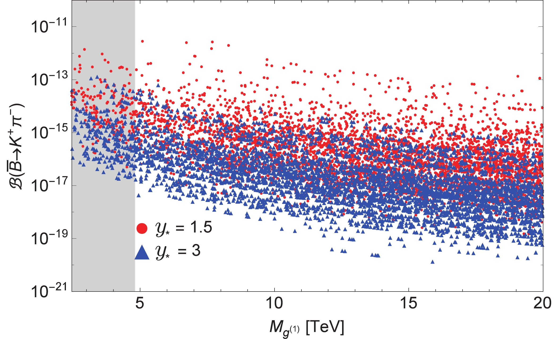
Figure 2. (color online) Predictions for the
$\smash{\overline B}^0\to K^+\pi^-$ branching ratio as a function of the KK gluon mass$M_{g^{(1)}}$ in the${{\rm{RS}}_c}$ model for two different values of$y_{\star}$ . The gray region is excluded by the analysis of the electroweak precision observables.The dominant contributions in the
$ {{\rm{RS}}_c} $ model come from the KK gluons. Observing the effects of the new heavy EW gauge bosons$ Z_H $ and$ Z^{\prime} $ on the$ \smash{\overline B}^0\to K^+\pi^- $ decay, we found, in agreement with [40], that imposing the$ \Delta m_K $ and$ \epsilon_K $ constraints,$ Z_H $ and$ Z^{\prime} $ give subleading contributions because the KK gluons still dominate the EW contributions in the$ (m_{12}^K)_{\rm{KK}} $ expression due to the strong RG enhancement of the$ C_4^{LR} $ coefficient. And the chiral enhancement of the$ {\cal{O}}_4 $ hadronic matrix element. In contrast, for the$ \Delta m_{B_d} $ constraint,$ Z_H $ and$ Z^{\prime} $ give comparable contributions to that of KK gluons because the RG enhancement of the$ C_4^{LR} $ coefficient is smaller and the chiral enhancement of the matrix elements of the$ LR $ type operators is absent. Despite the fact that the chiral enhancement of the matrix elements of the$ LR $ type operators in the$ B_d $ physics observables is absent, the matrix elements of the$ {\cal{O}}_4 $ and$ {\cal{\widetilde{O}}}_{4} $ operators with$ (S-P)(S+P) $ and$ (S+P)(S-P) $ structures are chirally enhanced in the PQCD formalism used for the amplitude of the$ \smash{\overline B}^0\to K^+\pi^- $ process. Also, as discussed previously, the WC's in the PQCD are calculated at the scale$ t $ of$ {\cal{O}}\sim (1-2) $ GeV, so that the RG enhancement is also large. Both of these factors play a role in increasing the$ \smash{\overline B}^0\to K^+\pi^- $ branching ratio in the$ {{\rm{RS}}_c} $ model, and together ensure that KK gluon contributions dominate over$ Z_H $ and$ Z^{\prime} $ contributions for a parameter point that satisfies the simultaneous constraints for$ \Delta m_K $ ,$ \epsilon_K $ and$ \Delta m_{B_d} $ .In Fig. 3, we show the predictions of the decay rate in the bulk-Higgs RS model for two representative values of
$ \beta $ , after simultaneously imposing the$ \Delta m_K $ ,$ \epsilon_K $ and$ \Delta m_{B_d} $ constraints. The red and blue scatter points again correspond to model points obtained using$ y_{\star} = 1.5 $ and 3, respectively. The gray shaded regions in Figs. 3(a) and 3(b) indicate the parameter space excluded by the analysis of the electroweak precision data for the cases of$ \beta = 1 $ and$ \beta = 10 $ . Here, we mention that while imposing the experimental constraints for$ \Delta m_K $ ,$ \epsilon_K $ and$ \Delta m_{B_d} $ , we set the required input parameters to their central values in both RS models and allow the resulting observables to deviate by ±50%, ±30% and ±30%, respectively, in analogy to the analysis in [40]. Again, we see in the figures that a large number of scatter points in the allowed parameter space lies in the central region for each value of$ M_{g^{(1)}} $ . In the case of$ y_{\star} = 3 $ , there are more elementary fermions such that their profiles are shifted towards the UV brane, which results in more suppressed FCNCs compared to the case of$ y_{\star} = 1.5 $ . Therefore, from Fig. 3, we see that the predictions of the$ \smash{\overline B}^0\to K^+\pi^- $ decay rates for the parameter points with$ y_{\star} = 1.5 $ are generally larger due to less suppressed FCNCs than for$ y_{\star} = 3 $ . However, the smaller$ y_{\star} $ are subjecte to more severe constraints from flavor observables. Hence, after applying the$ \Delta m_K $ ,$ \epsilon_K $ and$ \Delta m_{B_d} $ constraints simultaneously, the maximum possible predictions for$ y_{\star} = 1.5 $ move towards the case$ y_{\star} = 3 $ . Considering the maximum possible enhancement of the branching ratio in Fig. 3(a), we note that the$ y_{\star} = 3 $ case is subject to relatively less severe constraints from$ K^0-\smash{\overline K}^0 $ and$ B^0-\smash{\overline B}^0 $ mixing, and the branching ratio of$ {\cal{O}}(10^{-14}) $ is predicted for some parameter points. In the case of$ y_{\star} = 1.5 $ , the maximum possible branching ratio is of$ {\cal{O}}(10^{-13}) $ for a number of parameter points, which suggests an increase of six orders of magnitude above the SM prediction. Comparing the results for$ \beta = 10 $ with the scenario with$ \beta = 1 $ , we observe a wider range of predictions for both cases of$ y_{\star} $ in the case of$ \beta = 10 $ . The maximum possible branching ratios in both cases of$ y_{\star} $ move further above in the$ \beta = 10 $ scenario, but in general the order of magnitude for the branching ratio remains the same for both$ y_{\star} $ cases.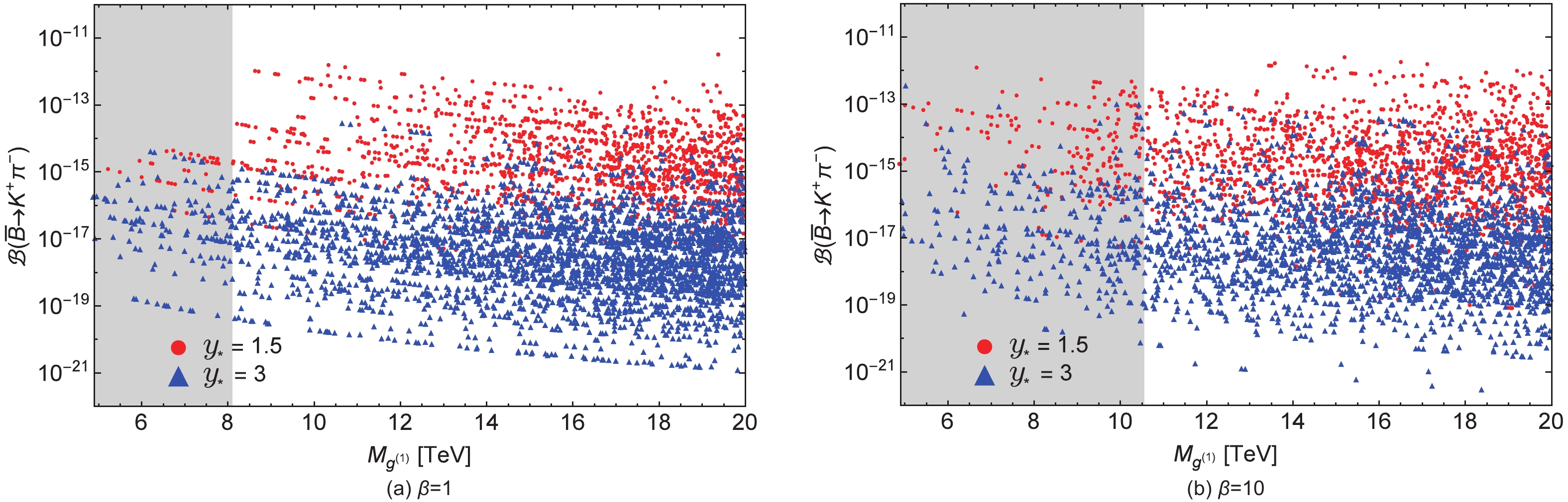
Figure 3. (color online) Predictions for the
$\smash{\overline B}^0\to K^+\pi^-$ branching ratio as a function of the KK gluon mass$M_{g^{(1)}}$ in the bulk-Higgs RS model with$\beta=1$ and$\beta = 10$ . The red and blue scatter points correspond to$y_{\star}=1.5$ and$3$ , respectively. The gray regions are excluded by the analysis of the electroweak precision observables. -
The doubly weak transition
$ b \to dd\bar s $ is highly suppressed in SM, which makes it sensitive to any new physics contributions beyond SM. In this paper, we studied the pure annihilation type rare two-body exclusive decay$ \smash{\overline B}^0\to K^+\pi^- $ , mediated by the$ b \to dd\bar s $ transition, in the PQCD framework. The wrong sign decay$ \smash{\overline B}^0\to K^+\pi^- $ can be distinguished from the right sign decay$ B^0\to K^+\pi^- $ by the time-dependent measurement of the neutral B decays through$ B^0-\smash{\overline B}^0 $ mixing. Therefore, we propose to perform a time-dependent analysis to search for the wrong sign$ \smash{\overline B}^0\to K^+\pi^- $ decay, which may expose possible NP effects.Starting with the most general local effective Hamiltonian for the
$ b \to dd\bar s $ processes, we analyzed the$ \smash{\overline B}^0\to K^+\pi^- $ decay in a model independent way, where the constraints on the Wilson coefficients of different new physics dimension-6 operators were obtained for a specific experimental precision for the observable$ R $ . Moreover, several examples of NP models, such as NP with conserved global charge, minimal flavor violation (MFV) and next-to-minimal flavor violation (NMFV), were discussed, and their predictions for the ratio$ R $ presented. In the case of NP with conserved charge we pointed out that due to the hierarchies among the NP couplings, the ratio$ R_X $ in different NP scenarios can be very large, after satisfying the bounds from$ K^0-\smash{\overline K}^0 $ and$ B^0-\smash{\overline B}^0 $ mixing. This mechanism represents a generalization of the sneutrino exchange in R-parity violating supersymmetry. Furthermore, sizable enhancement of the ratio$ R $ is possible in NMFV models in the presence of different new physics dimension-6 operators.We also presented the results for the
$ \smash{\overline B}^0\to K^+\pi^- $ branching fraction in two types of RS models, after considering all relevant constraints. In both models, the main contribution to the decay rate comes from the tree level exchanges of KK gluons such that, after satisfying the$ \Delta m_K $ ,$ \epsilon_K $ and$ \Delta m_{B_d} $ constraints simultaneously, for the case of the$ {{\rm{RS}}_c} $ model with$ y_{\star} = 1.5 $ , a maximum increase of six orders of magnitude of the branching fraction is possible for a few parameter points. Similarly, in the bulk-Higgs RS model, after considering all relevant constraints, the maximum possible enhancement of five and six orders of magnitude is probable for$ y_{\star} = 3 $ and$ y_{\star} = 1.5 $ , respectively, for both broad and narrow Higgs profile cases. This decay is therefore interesting for search of new physics in future experiments.We are grateful to Qin Qin, Wei Wang, Qi-An Zhang, Jing-Bin Liu and Chao Wang for useful discussions.
-
The wave functions describe the hadronization of a quark and anti-quark into a meson
$ M $ , which is a non-perturbative but universal process. For the incoming$ B $ meson, the wave function is written as$ \tag{A1}\Phi_{B,\alpha\beta}(x,b) = \frac{i}{\sqrt{2N_c}} \left[(\not \!\!P_1 \gamma_5)_{\alpha\beta}+ m_B \gamma_{5\alpha\beta}\right] \phi_B(x,b), $

where
$ N_c = 3 $ is the color degree of freedom, and$ P_1 $ is its momentum. For$ \phi_B $ , the model wave function was proposed in [27-29,31]$\tag{A2} \phi_B(x,b) = N_Bx^2(1-x)^2 \exp\left[-\frac{1}{2}\left(\frac{xm_B}{\omega_B}\right)^2-\frac{\omega_B^2 b^2}{2}\right] \;, $

where the normalization constant
$ N_B $ is related to the decay constant$ f_B $ through$\tag{A3} \int_0^1 {\rm d}x\, \phi_B(x,b = 0) = \frac{f_B}{2\sqrt{2N_c}}\;. $

The wave functions of the outgoing kaon and pion, up to twist-3 accuracy, with momenta respectively
$ P_2 $ and$ P_3 $ , are defined as [52,53]$\tag{A4} \begin{split} \langle K^+(P_2)|\bar u_{\beta}(0)s_{\alpha}(z)|0\rangle = &-\frac{i}{\sqrt{2N_c}}\int_0^1 {\rm{d}}x_2\, {\rm{e}}^{{\rm i}x_2P_2.z} \{\gamma_5 {\not \!\! P}_2 \phi_K^A(x_2)\\&+\gamma_5 m_{0K} \phi_K^P(x_2) -m_{0K}\gamma_5({\not \! n}{\not \! \nu}-1) \phi_K^{T}(x_2) \}_{\alpha\beta}, \end{split} $

$ \tag{A5}\begin{split} \langle \pi^-(P_3)|\bar d_{\beta}(0)u_{\alpha}(z)|0\rangle =& -\frac{i}{\sqrt{2N_c}}\int_0^1 {\rm{d}}x_3\, {\rm{e}}^{{\rm i}x_3P_3.z} \{\gamma_5 {\not \!\! P}_3 \phi_{\pi}^A(x_3)\\&+\gamma_5 m_{0\pi} \phi_{\pi}^P(x_3) -m_{0\pi}\gamma_5({\not \! \nu}{\not \! n}-1) \phi_{\pi}^{T}(x_3) \}_{\alpha\beta}, \end{split} $

where
$ n = (1,0,{\bf 0}_T )\propto P_2 $ ,$ v = (0,1,{\bf 0}_T) \propto P_3 $ , and the chiral masses are$\tag{A6} \begin{aligned} m_{0K} = \frac{m_K^2}{m_u + m_s},\,\,\,m_{0\pi} = \frac{m_\pi^2}{m_u + m_d}. \end{aligned} $

The light-cone distribution amplitudes
$ \phi^A_{\pi(K)} $ ,$ \phi_{\pi(K)}^P $ and$ \phi_{\pi(K)}^T $ have been studied within the QCD sum rules [52-54], and they are expanded in the Gegenbauer polynomials,$\tag{A7} \begin{split} \phi_{\pi(K)}^A(x) = & \frac{f_{\pi(K)}}{2\sqrt{2N_c}} 6x(1-x) \left[1 + a_1^{\pi(K)} C_1^{3/2}(t) \right.\\&\left.+a_2^{\pi(K)}C_2^{3/2}(t) +a_4^{\pi(K)}C_4^{3/2}(t)\right] \;, \end{split} $

$ \tag{A8}\begin{split} \phi^P_{\pi(K)}(x) = & \frac{f_{\pi(K)}}{2\sqrt{2N_c}}\, \bigg[ 1 +\left(30\eta_3 -\frac{5}{2}\rho_{\pi(K)}^2\right) C_2^{1/2}(t) \\&- 3\left\{ \eta_3\omega_3 + \frac{9}{20}\rho_{\pi(K)}^2(1+6a_2^{\pi(K)}) \right\} C_4^{1/2}(t) \bigg]\;, \end{split} $

$\tag{A9} \begin{split} \phi^T_{\pi(K)}(x) = & \frac{f_{\pi(K)}}{2\sqrt{2N_c}}\, (1-2x)\bigg[ 1 + 6\left(5\eta_3 -\frac{1}{2}\eta_3\omega_3 - \frac{7}{20} \rho_{\pi(K)}^2 \right.\\&\left.- \frac{3}{5}\rho_{\pi(K)}^2 a_2^{\pi(K)} \right) (1-10x+10x^2) \bigg]\;, \end{split} $

with
$ \rho_{\pi(K)}\equiv m_{\pi(K)}/m_{0\pi(K)} $ . The Gegenbauer polynomials are defined as$\tag{A10} \begin{split} C_2^{1/2}(t)\, =& \, \frac{1}{2} \left(3\, t^2-1\right) \;, C_4^{1/2}(t)\, = \, \frac{1}{8} \left(3-30\, t^2+35\, t^4\right) \;, \\ C_1^{3/2}(t)\, =& \, 3\, t \;, C_2^{3/2}(t)\, = \, \frac{3}{2} \left(5\, t^2-1\right) \;, C_4^{3/2}(t) \, = \, \frac{15}{8} \left(1-14\, t^2+21\, t^4\right) \;, \end{split} $

with
$ t = 2x-1 $ . For the other parameters, such as$ a_i $ ,$ \eta_i $ and$ \omega_i $ , we refer the reader to [4]. -
First, we present the auxiliary functions as
$ \tag{B1}G_0^2 = (1-x_{2})x_{3}m^2_{B}, $

$\tag{B2} G_a^2 = x_3 m^2_{B}, $

$\tag{B3}G_b^2 = (1-x_2)m^2_{B}, $

$\tag{B4} G_c^2 = (1-x_2)(x_1-x_3)m^2_{B}, $

$\tag{B5}G_d^2 = (1-x_2(1-x_1-x_3))m^2_{B}. $

The hard scale
$ t $ in the amplitudes is selected as the largest energy scale:$ \tag{B6} t_{a} = \max\Big\{\sqrt{|G_0^2|},\sqrt{|G_a^2|}, 1/b_{2},1/b_{3}\Big\}, $

$\tag{B7} t_{b} = \max\Big\{\sqrt{|G_0^2|},\sqrt{|G_b^2|}, 1/b_{2},1/b_{3}\Big\}, $

$\tag{B8} t_{c} = \max\Big\{\sqrt{|G_0^2|},\sqrt{|G_c^2|}, 1/b_{1},1/b_{3}\Big\}, $

$\tag{B9} t_{d} = \max\Big\{\sqrt{|G_0^2|},\sqrt{|G_d^2|}, 1/b_{1},1/b_{3}\Big\}. $

By inserting the different operators, we calculate the amplitudes for the factorizable annihilation diagram in Fig. 1(a) and (b) and obtain
$\tag{B10} \begin{split} F_{a1} =& 4\pi C_F m_B^2f_B \int_0^1 {\rm d}x_2 {\rm d}x_3 \int_0^{\infty} b_2 {\rm d}b_2 b_3 {\rm d}b_3 \bigg[\Big\{x_3 \phi_{K}^A(x_2)\phi_{\pi}^A(x_3) \\ &+2r_{\pi}r_K \phi_{K}^P(x_2)\Big[\left(\phi_{\pi}^P(x_3)-\phi_{\pi}^T(x_3)\right) +x_3\left(\phi_{\pi}^P(x_3)+\phi_{\pi}^T(x_3)\right)\Big] \Big\} \\ &\times E_{a}(t_a)h_a(x_2,x_3,b_2,b_3)S_t(x_3)-\Big\{(1-x_2)\phi_{K}^A(x_2)\phi_{\pi}^A(x_3)\\&+4r_{\pi}r_K \phi_{K}^P(x_2)\phi_{\pi}^P(x_3) -2r_{\pi}r_K x_2 \phi_{\pi}^P(x_3)\left(\phi_{K}^P(x_2)-\phi_{K}^T(x_2)\right)\Big\}\\&\times E_{a}(t_b)h_b(x_2,x_3,b_2,b_3)S_t(x_2)\bigg], \end{split} $

$\tag{B11} \begin{split} F_{a2} =& 4\pi C_F m_B^2f_B \int_0^1 {\rm d}x_2 {\rm d}x_3 \int_0^{\infty} b_2 {\rm d}b_2 b_3 {\rm d}b_3 \bigg[\Big\{2r_{K}\phi_{K}^P(x_2)\phi_{\pi}^A(x_3) \\ &+r_{\pi} x_3\phi_{K}^A(x_2)\left(\phi_{\pi}^P(x_3)-\phi_{\pi}^T(x_3)\right)\Big\}E_{a}(t_a)h_a(x_2,x_3,b_2,b_3)S_t(x_3) \\ &+\Big\{r_{K}(1-x_2)\phi_{\pi}^A(x_3)\left(\phi_{K}^P(x_2)+\phi_{K}^T(x_2)\right) \\ &+2r_{\pi}\phi_{K}^A(x_2)\phi_{\pi}^P(x_3)\Big\} E_{a}(t_b)h_b(x_2,x_3,b_2,b_3)S_t(x_2)\bigg], \end{split} $

$\tag{B12} \begin{split} &F_{a3} = -\frac{1}{2}F_{a2}, \qquad F_{a4} = F_{a2},\\& \quad\qquad F_{a5} = -\frac{1}{2}F_{a1}, \end{split} $

where
$ C_F = 4/3 $ is the group factor of the$ {SU}(3)_c $ gauge group, and$ r_i = m_{0i}/M_B $ ($ i = K,\pi $ ). The threshold resummation$ S_t(x) $ is parameterized as [32]$\tag{B13} \begin{aligned} S_t(x) = \frac{2^{1+2c}\Gamma(3/2 +c)}{\sqrt{\pi} \Gamma(1+c)} \left[x(1-x)\right]^c,\quad c = 0.3. \end{aligned} $

The amplitudes for the nonfactorizable annihilation diagram in Fig. 1(c) and 1(d) are given by
$\tag{B14} \begin{split} {\cal{M}}_{a1}\! \!=\!& 8\pi C_F \frac{\sqrt{2N_c}}{N_c} m_B^2 \!\!\int_0^1\!\!\! {\rm d}x_1 {\rm d}x_2 {\rm d}x_3 \int_0^{\infty}\!\!\!b_1 {\rm d}b_1 b_3 {\rm d}b_3 \phi_B \bigg[\Big\{(1\!\!-\!\!x_2) \phi_{K}^A(x_2)\phi_{\pi}^A(x_3) \\ &+r_{\pi}r_K \Big[(1\!\!-\!\!x_2)(\phi_{K}^P(x_2)-\phi_{K}^T(x_2))(\phi_{\pi}^P(x_3)\!+\!\phi_{\pi}^T(x_3))\!+\!x_3(\phi_{K}^P(x_2)\!+\!\phi_{K}^T(x_2)) \\ &\times(\phi_{\pi}^P(x_3)-\phi_{\pi}^T(x_3))\Big]\Big\} E_{a}^{\prime}(t_c)h_c(x_1,x_2,x_3,b_1,b_3)-\Big\{x_3\phi_{K}^A(x_2)\phi_{\pi}^A(x_3) \\ &+r_{\pi}r_K\Big[4\phi_{K}^P(x_2)\phi_{\pi}^P(x_3)-(1-x_3)(\phi_{K}^P(x_2)-\phi_{K}^T(x_2))(\phi_{\pi}^P(x_3)+\phi_{\pi}^T(x_3)) \\ &-x_2(\phi_{K}^P(x_2)+\phi_{K}^T(x_2))(\phi_{\pi}^P(x_3)-\phi_{\pi}^T(x_3))\Big]\Big\} \\&\times E_{a}^{\prime}(t_d)h_d(x_1,x_2,x_3,b_1,b_3)\bigg]. \end{split} $

$\tag{B15} \begin{split} {\cal{M}}_{a2}& = 4\pi C_F \frac{\sqrt{2N_c}}{N_c} m_B^2 \int_0^1 {\rm d}x_1 {\rm d}x_2 {\rm d}x_3 \int_0^{\infty} b_1 {\rm d}b_1 b_3 {\rm d}b_3 \phi_B \bigg[\Big\{r_K(1-x_2)\\ &\times\phi_{\pi}^A(x_3)(\phi_{K}^P(x_2)+\phi_{K}^T(x_2))+2r_{\pi}x_3\phi_{K}^A(x_2)\phi_{\pi}^P(x_3)\Big\}E_{a}^{\prime}(t_c)\\ &\times h_c(x_1,x_2,x_3,b_1,b_3)+\Big\{r_K\phi_{\pi}^A(x_3)(\phi_{K}^P(x_2)+\phi_{K}^T(x_2))\\&-2r_K x_2\phi_{\pi}^A(x_3)\phi_{K}^P(x_2) +r_{\pi}\phi_{K}^A(x_2)\Big[(\phi_{\pi}^P(x_3)+\phi_{\pi}^T(x_3))+x_3(\phi_{\pi}^P(x_3)\\&-\phi_{\pi}^T(x_3))\Big] \Big\}E_{a}^{\prime}(t_d)h_d(x_1,x_2,x_3,b_1,b_3)\bigg]. \end{split} $

$\tag{B16} \begin{split} {\cal{M}}_{a3}=& 4\pi C_F \frac{\sqrt{2N_c}}{N_c} m_B^2 \int_0^1 {\rm d}x_1 {\rm d}x_2 {\rm d}x_3 \int_0^{\infty} b_1 {\rm d}b_1 b_3 {\rm d}b_3 \phi_B \\&\times\bigg[\Big\{-2r_K(1-x_2)\phi_{K}^P(x_2)\phi_{\pi}^A(x_3)\\ &+r_{\pi}x_3\phi_{K}^A(x_2)(\phi_{\pi}^T(x_3)-\phi_{\pi}^P(x_3))\Big\}E_{a}^{\prime}(t_c)h_c(x_1,x_2,x_3,b_1,b_3) \\ &+\Big\{r_Kx_2\phi_{\pi}^A(x_3)(\phi_{K}^P(x_2)+\phi_{K}^T(x_2))-2r_K\phi_{\pi}^A(x_3)\phi_{K}^P(x_2) \\ &+r_{\pi}\phi_{K}^A(x_2)(\phi_{\pi}^P(x_3)+\phi_{\pi}^T(x_3))-2r_{\pi}x_3\phi_{K}^A(x_2)\phi_{\pi}^P(x_3)\Big\}\\&\times E_{a}^{\prime}(t_d)h_d(x_1,x_2,x_3,b_1,b_3)\bigg]. \end{split} $

$\tag{B17} \begin{split} {\cal{M}}_{a4} =& -4\pi C_F \frac{\sqrt{2N_c}}{N_c} m_B^2 \int_0^1\!\! {\rm d}x_1 {\rm d}x_2 {\rm d}x_3 \int_0^{\infty} \!\!b_1 {\rm d}b_1 b_3 {\rm d}b_3 \phi_B \bigg[\Big\{x_3\phi_{K}^A(x_2)\phi_{\pi}^A(x_3)\\ &+r_{\pi}r_K \Big[x_3(\phi_{K}^P(x_2)-\phi_{K}^T(x_2))(\phi_{\pi}^P(x_3)+\phi_{\pi}^T(x_3))\\ &+(1-x_2)(\phi_{K}^P(x_2)+\phi_{K}^T(x_2))(\phi_{\pi}^P(x_3)-\phi_{\pi}^T(x_3))\Big]\Big\}E_{a}^{\prime}(t_c)\\ &\times h_c(x_1,x_2,x_3,b_1,b_3)-\Big\{(1\!-\!x_2)\phi_{K}^A(x_2)\phi_{\pi}^A(x_3)\!-\!r_{\pi}r_K\Big[\!-4\phi_{K}^P(x_2)\phi_{\pi}^P(x_3)\\ &+x_2(\phi_{K}^P(x_2)-\phi_{K}^T(x_2))(\phi_{\pi}^P(x_3)+\phi_{\pi}^T(x_3))+(1-x_3)\\ &\times(\phi_{K}^P(x_2)+\phi_{K}^T(x_2))(\phi_{\pi}^P(x_3)-\phi_{\pi}^T(x_3))\Big]\Big\}E_{a}^{\prime}(t_d)h_d(x_1,x_2,x_3,b_1,b_3)\bigg]. \end{split} $

$\tag{B18} \begin{split} {\cal{M}}_{a5} =& -4\pi C_F \frac{\sqrt{2N_c}}{N_c} m_B^2 \int_0^1 {\rm d}x_1 {\rm d}x_2 {\rm d}x_3 \int_0^{\infty} b_1 {\rm d}b_1 b_3 {\rm d}b_3 \phi_B \bigg[\Big\{-r_K(1-x_2) \\ &\times\phi_{\pi}^A(x_3)(\phi_{K}^P(x_2)-\phi_{K}^T(x_2))+r_{\pi}x_3\phi_{K}^A(x_2) (\phi_{\pi}^P(x_3)+\phi_{\pi}^T(x_3))\Big\} \\ &\times E_{a}^{\prime}(t_c)h_c(x_1,x_2,x_3,b_1,b_3)-\Big\{ r_K(1+x_2)\phi_{\pi}^A(x_3)(\phi_{K}^P(x_2)-\phi_{K}^T(x_2)) \\ &+r_{\pi}(x_3-2)\phi_{K}^A(x_2) (\phi_{\pi}^P(x_3)+\phi_{\pi}^T(x_3)) \Big\} E_{a}^{\prime}(t_d)h_d(x_1,x_2,x_3,b_1,b_3)\bigg]. \end{split} $

In the above formulas, the functions
$ E_{a}(t) $ and$ E_{a}^{\prime}(t) $ are$\tag{B19} \begin{split} E_{a}(t) =& \alpha_s(t)\exp[-S_{K}(t)-S_{\pi}(t)];\\ E_{a}^{\prime}(t) =& \alpha_s(t)\exp[-S_{B}(t)-S_{K}(t)-S_{\pi}(t)]|_{b_2 = b_3}. \end{split} $

$ S_B $ ,$ S_K $ , and$ S_\pi $ result from resummation of doubly logarithms caused by the overlap of soft collinear gluon corrections and single logarithms due to the renormalization of ultra-violet divergence [33], which are defined as$ \tag{B20} S_B(t) = s(x_1P_1^+,b_1) + \frac{5}{3} \int_{1/b_1}^t \frac{{\rm d}\mu'}{\mu'} \gamma_q(\mu'), $

$ \tag{B21} S_K(t) = s(x_2P_2^+,b_2)+s((1-x_2)P_2^+,b_2)+2 \int_{1/b_2}^t \frac{{\rm d}\mu'}{\mu'} \gamma_q(\mu'), $

$\tag{B22} S_\pi(t) = s(x_3P_3^-,b_3)+s((1-x_3)P_3^-,b_3)+2 \int_{1/b_3}^t \frac{{\rm d}\mu'}{\mu'} \gamma_q(\mu'). $

$ s(Q,b) $ , the so-called Sudakov factor, is given as [55]$ \tag{B23}\begin{split} s(Q,b) = & \int_{1/b}^Q \!\! \frac{{\rm d}\mu'}{\mu'} \left[\left\{\frac{2}{3}(2\gamma_E-1-\log 2)+C_F \log \frac{Q}{\mu'} \right\} \frac{\alpha_s(\mu')}{\pi} \right. \\ & \left.+ \left\{ \frac{67}{9} - \frac{\pi^2}{3} - \frac{10}{27} n_f + \frac{2}{3} \beta_0 \log \frac{\gamma_E}{2} \right\} \left( \frac{\alpha_s(\mu')}{\pi} \right)^2 \log \frac{Q}{\mu'} \right], \end{split} $

where
$ \gamma_E $ is the Euler constant, and$ \gamma_q = \alpha_s/\pi $ is the quark anomalous dimension. For the strong coupling constant, we use$ \tag{B24} \alpha_s(\mu) = \frac{4 \pi}{\beta_0 \log (\mu^2 / \Lambda^2)}, $

where
$ \beta_0 = (33-2n_f)/3 $ , and$ n_f $ is the number of active flavors.$ \Lambda = 250 {\rm MeV} $ is QCD scale at$ n_f = 4 $ .The functions
$ h_i $ ($ i = a,b,c,d $ ) in the decay amplitudes arise from the propagators of the virtual quarks and gluons, which are expressed by$\tag{B25} \begin{split} h_a(x_2,x_3,b_2,b_3) =& \left( \frac{\pi i}{2}\right)^2 H_0^{(1)}\left(\sqrt{G_0^2}\, b_2\right) \\&\times\left\{H_0^{(1)}\left(\sqrt{G_a^2}\, b_2\right)J_0\left(\sqrt{G_a^2}\, b_3\right) \theta(b_2 - b_3) + (b_2 \leftrightarrow b_3 ) \right\}, \end{split} $

$\tag{B26} \begin{split} h_b(x_2,x_3,b_2,b_3) =& \left( \frac{\pi i}{2}\right)^2 H_0^{(1)}\left(\sqrt{G_0^2}\, b_3\right) \\&\times\left\{H_0^{(1)}\left(\sqrt{G_b^2}\, b_2\right)J_0\left(\sqrt{G_b^2}\, b_3\right) \theta(b_2 - b_3) + (b_2 \leftrightarrow b_3 ) \right\}, \end{split} $

$\tag{B27} \begin{split} h_c(x_1,x_2,x_3,b_1,b_3) =& \biggl\{ \frac{\pi i}{2} {\rm{H}}_0^{(1)}(\sqrt{G_0^2}\, b_1) {\rm{J}}_0(\sqrt{G_0^2}\, b_3) \theta(b_1-b_3)+ (b_1 \leftrightarrow b_3) \biggr\}\\ & \times\left( \begin{matrix} {\rm{K}}_0(\sqrt{G_c^2} b_1), & {\rm{for}}\quad G_c^2>0 \\ \displaystyle\frac{\pi i}{2} {\rm{H}}_0^{(1)}(\sqrt{|G_c^2|}\ b_1), & {\rm{for}}\quad G_c^2<0 \end{matrix}\right), \end{split} $

$\tag{B28} \begin{split} h_d(x_1,x_2,x_3,b_1,b_3) = &\biggl\{ \frac{\pi i}{2} {\rm{H}}_0^{(1)}(\sqrt{G_0^2}\, b_1) {\rm{J}}_0(\sqrt{G_0^2}\, b_3) \theta(b_1-b_3)+ (b_1 \leftrightarrow b_3) \biggr\}\\ & \times\left( \begin{matrix} {\rm{K}}_0(\sqrt{G_d^2} b_1), & {\rm{for}}\quad G_d^2>0 \\ \displaystyle\frac{\pi i}{2} {\rm{H}}_0^{(1)}(\sqrt{|G_d^2|}\ b_1), & {\rm{for}}\quad G_d^2<0 \end{matrix}\right), \end{split} $

where
$ {\rm{H}}_0^{(1)}(z) = {\rm{J}}_0(z) + i\, {\rm{Y}}_0(z) $ .
New physics search in the doubly weak decay ${{\overline B}^0 \to K^+ \pi^- }$
- Received Date: 2018-12-17
- Accepted Date: 2019-04-11
- Available Online: 2019-07-01
Abstract: The doubly weak transition


 DownLoad: