


 Abstract
 HTML
HTML Reference
 Related
 PDF
PDF


-
The quantum field theory entanglement is widely studied in the literature [1-3]. Recently, the source of entanglement entropy was likewise considered in [4]. It expresses the vacuum state in terms of the superposition of particle pair states in the configuration space by the Bogoliubov transformation, which transforms the original degrees of freedom to actual local degrees of freedom. Interestingly, it tells us that the entanglement entropy originates from the particle pairs across the boundary. The area law [1, 5-7] emerges naturally by this method. In [4], only the free scalar field is discussed. In this study, we generalize it to 1+1 and 2+1 dimensional Majorana (spin-
$ \displaystyle\frac{1}{2} $ ) field, 2+1 dimensional U(1) gauge (free spin-1) field, and 3+1 dimensional weak gravitational (free massless spin-2) field. Because there is a Hilbert space with a tensor product structure for the spin-$ \displaystyle\frac{1}{2} $ field, the generalization is straight forward. As for higher spin fields, more treatments are required because of the gauge redundancy.The definition of entanglement entropy in gauge theory was discussed in [8, 9]. The definition of entanglement entropy is heavily dependent on the tensor product structure of the Hilbert space. However, because of the gauge redundancy, there is no natural structure as such in the Hilbert space of the gauge field. Some studies addressed the entanglement entropy of the gauge field with various prescriptions [10, 11], which give up the direct tensor product structure and introduced a "center". It is clear that this issue is also present in the gravitational theories [12, 13], as gravitational theories likewise are gauge theories. The tensor product structure problem of gravitational theories is still under discussion [14]. In this study, we deal with the gauge redundancy by the light-cone gauge for both the free U(1) gauge field and the gravitational field (or strictly speaking, a free spin-2 field). We demonstrate that this gauge-fixing provides a natural tensor product structure in the Hilbert spaces belonging to them, while surrendering the explicit Lorentz invariance.
Imposing the light-cone gauge, we find that the Lagrangian of the U(1) gauge field and gravitational field simplifies significantly and behaves like a massless scalar field. Subsequently, we quantize them and obtain their Hilbert spaces with the tensor product structure. We perform the Bogoliubov transformation of the theories and express the ground state in terms of a local basis of degrees of freedom. Finally, we calculate the second Rényi entropy, which is a good approximation of the entanglement entropy. We find that in such a prescription, the area law is also naturally preserved.
Our paper is organized as follows. In Section 2, we make a Bogoliubov transformation of the 1+1 dimensional Majorana field and consider its second Rényi entropy. In Section 3, we perform this procedure for the 2+1 dimensional Majorana field. In Section 4, we derive the Lagrangian of the 2+1 dimensional free U(1) gauge field in the light-cone gauge and obtain its Hilbert space with the natural tensor product structure. Then we perform a Bogoliubov transformation and calculate the second Rényi entropy. In Section 5, we generalize our method to the 3+1 dimensional gravitational (free spin-2) field in the light-cone gauge. In Section 6, we provide conclusions of our work.
-
The Majorana field
$ \psi $ is a field sharing the same Lagrangian with the Dirac field, but satisfying the condition$ \psi^\ast=\psi $ , which means that the anti-particle and particle of the Majorana field are the same [15]. In 1+1 dimensions at t = 0, a Majorana field with$ \gamma^\mu=(\sigma_y,i\sigma_x) $ has the form [16]$ \begin{split} \psi (x) = &\int {\frac{{\rm d}k}{{\sqrt {2\pi } }}} \frac{1}{{\sqrt {2\omega } }}\left[ {\frac{1}{{\sqrt {\omega + k} }}\left( {\begin{array}{*{20}{c}} {\omega + k}\\ {i\mu } \end{array}} \right){b_k} }\right.\\&+\left.{ \frac{1}{{\sqrt {\omega - k} }}\left( {\begin{array}{*{20}{c}} {\omega - k}\\ { - i\mu } \end{array}} \right)b_{ - k}^\dagger } \right]{{\rm e}^{{\rm i}kx}}, \end{split} $

(1) where the annihilation and creation operators bk and
$ b_p^\dagger $ satisfy the anti-commutation relation$ \{b_k,b_p^\dagger\}=\delta(k-p) $ . We define the vacuum$ |0\rangle $ as the vacuum of this set of operators, i.e.$ b_k|0\rangle=0 $ .Let us consider the following Bogoliubov transformation [17]
$\psi (x) = \int {\frac{{\rm d}k}{{\sqrt {2\pi } }}} \left( {\begin{array}{*{20}{c}} {{a_{1k}}}\\ {{a_{2k}}} \end{array}} \right){{\rm e}^{{\rm i}kx}},$

(2) which transforms the operators
$ (b_k,b_{-k}^\dagger) $ into the new set of operators$ (a_{1k},a_{2k}) $ . For the Majorana field, we have the relation$\{ {\psi _\alpha }(x),{\psi _\beta }(y)\} = {\delta _{\alpha \beta }}\delta (x - y).$

(3) where
$ \alpha,\beta=0,1 $ represent the two components of the Majorana field. To satisfy (3), the operators$ a_{1k} $ and$ a_{2p} $ should have the relation$\{ {a_{ik}},{a_{jp}}\} = {\delta _{ij}}\delta (k + p),$

(4) where
$ i,j=1,2 $ . We choose${a_{1k}} = \frac{1}{{\sqrt 2 }}\left({a_k} + a_{ - k}^\dagger \right),$

(5) ${a_{2k}} = - i\frac{1}{{\sqrt 2 }}\left({a_k} - a_{ - k}^\dagger \right),$

(6) where
$ (a_k,a_{-k}^\dagger) $ are new annihilation and creation operators that satisfy the anti-commutation relation$ \{a_k, a_p^\dagger\}= $ $\delta(k-p) $ . We can verify that (5) and (6) satisfy the constraint (4). We define the vacuum$ |\Omega\rangle $ , which is annihilated by ak, i.e.$ a_k|\Omega\rangle=0 $ . Hence, we obtain the Bogoliubov transformation between$ (a_k,a_{-k}^\dagger) $ and$ (b_k,b_{-k}^\dagger) $ $ \begin{split} \left( {\begin{array}{*{20}{c}} {{b_k}}\\ {b_{ - k}^\dagger } \end{array}} \right) =& \frac{1}{{2\sqrt \omega }}\left( {\begin{array}{*{20}{c}} {\sqrt {\omega + k} - \sqrt {\omega - k} }&{\sqrt {\omega + k} + \sqrt {\omega - k} }\\ {\sqrt {\omega + k} + \sqrt {\omega - k} }&{\sqrt {\omega - k} - \sqrt {\omega + k} } \end{array}} \right) \\&\times \left( {\begin{array}{*{20}{c}} {{a_k}}\\ {a_{ - k}^\dagger } \end{array}} \right). \end{split} $

(7) Certainly, we have
${b_k} = \frac{1}{{2\sqrt \omega }}\left(\left(\sqrt {\omega + k} - \sqrt {\omega - k} \right){a_k} + \left(\sqrt {\omega + k} + \sqrt {\omega - k} \right)a_{ - k}^\dagger \right).$

(8) Because we have
$ b_k|0\rangle=0 $ , the new set of operators satisfy$\left(\left(\sqrt {\omega + k} - \sqrt {\omega - k} \right){a_k} + \left(\sqrt {\omega + k} + \sqrt {\omega - k} \right)a_{ - k}^\dagger \right)|0\rangle = 0.$

(9) The vacuum
$ |0\rangle $ can be expressed as a state constructed from the new set of operators$\begin{array}{*{20}{l}} {\left| 0 \right\rangle }&{ = \displaystyle\frac{1}{\gamma }{{\rm e}^{ - \sum\limits_k {{C_k}} a_k^\dagger a_{ - k}^\dagger }}\left| \Omega \right\rangle } \end{array}\quad\quad\quad\quad\quad$

(10) $\quad = \frac{1}{\gamma }\prod\limits_k {\left( {1 - {C_k}a_k^\dagger a_{ - k}^\dagger } \right)} \left| \Omega \right\rangle ,\;\;$

(11) where
$ \gamma $ is the normalization factor,$ \left| \Omega \right \rangle $ is the vacuum defined by$ a_k \left| \Omega \right \rangle = 0 $ and the coefficient Ck is fixed by${C_k} = \frac{{\sqrt {\omega + k} + \sqrt {\omega - k} }}{{\sqrt {\omega + k} - \sqrt {\omega - k} }} = \frac{{\omega + \mu }}{k}.$

(12) Following [4], let us consider a system with a finite number of sites. The inverse Fourier transform of the operator ak is
${a_k} = \sum\limits_N {{a_N}} {{\rm e}^{- {\rm i}kN}},$

(13) where N is the site label. The vacuum
$ \left| \Psi \right \rangle\equiv\left| 0 \right \rangle $ of the operator bk can thus be written as$\begin{split} \left| \Psi \right\rangle =& \displaystyle\frac{1}{\gamma }\prod\limits_k {\left( {1 - \sum\limits_{N,L} {{C_k}} {{\rm e}^{{\rm i}k(N - L)}}a_N^\dagger a_L^\dagger } \right)} \left| \Omega \right\rangle \\ \simeq & \displaystyle\frac{1}{\gamma }\left( {1 - \sum\limits_k {\sum\limits_{N,L} {{C_k}} } f_{NL}^ka_N^\dagger a_L^\dagger } \right)\left| \Omega \right\rangle , \end{split}$

(14) where
$f^k_{NL}={\rm e}^{{\rm i}k(N-L)}$ . To compute the entanglement entropy, the configuration space is divided into two regions A and$\bar{A}$ , where the sites in each region are labelled by small letters (n) and small letters with bar ($\bar{n}$ ), respectively. The region A we choose can be any subregion of the total system. The state$\left| \Psi \right \rangle$ is$ \begin{split} \left| \Psi \right\rangle \simeq \frac{1}{\gamma }\left(1 - \sum\limits_k {\sum\limits_{nl} {{C_k}} } f_{nl}^ka_n^\dagger a_l^\dagger - \sum\limits_k {\sum\limits_{\bar n\bar l} {{C_k}} } f_{\bar n\bar l}^ka_{\bar n}^\dagger a_{\bar l}^\dagger \right.\left. - \frac{1}{2}\sum\limits_k {\sum\limits_{\bar nl} {{C_k}} } \tilde f_{\bar nl}^ka_{\bar n}^\dagger a_l^\dagger \right)\left| \Omega \right\rangle , \end{split} $

(15) where
$ \tilde{f}^k_{\bar{n}l} = f^k_{\bar{n}l} + f^k_{l\bar{n}} $ .A reduced density matrix of
$ \rho_{A} $ is constructed by tracing out the degrees of freedom in region$ \bar{A} $ .$\begin{split} {\rho _A} =& {\rm{T}}{{\rm{r}}_{\bar A}}\left( {\left| \Psi \right\rangle \langle \Psi |} \right) \simeq \frac{1}{{{\gamma ^2}}}{\left[ {\left( {1 - \sum\limits_k {\sum\limits_{nl} {{C_k}} } f_{nl}^ka_n^\dagger a_l^\dagger } \right){{\left| \Omega \right\rangle }_{AA}}\langle \Omega |\left( {1 - \sum\limits_{k'} {\sum\limits_{n'l'} {C_{k'}^*} } f_{n'l'}^{*k'}{a_{n'}}{a_{l'}}} \right)} \right]{_{\bar A}}{\left\langle {\Omega |\Omega } \right\rangle _{\bar A}}}\\ & + {\left| \Omega \right\rangle _{AA}}\langle \Omega |\left[ {_{\bar A}\langle \Omega |\left( {\sum\limits_{k'} {\sum\limits_{\bar n'\bar l'} {C_{k'}^*} } f_{\bar n'\bar l'}^{*k'}{a_{\bar l'}}{a_{\bar n'}}} \right)\left( {\sum\limits_k {\sum\limits_{\bar n\bar l} {{C_k}} } f_{\bar n\bar l}^ka_{\bar n}^\dagger a_{\bar l}^\dagger } \right){{\left| \Omega \right\rangle }_{\bar A}}} \right] \\&+ a_l^\dagger {\left| \Omega \right\rangle _{AA}}\langle \Omega |{a_{l'}}\left[ {_{\bar A}\langle \Omega |\left( {\sum\limits_{k'} {\sum\limits_{\bar n'l'} {C_{k'}^*} } \tilde f_{\bar n'l'}^{*k'}{a_{\bar n'}}} \right)\left( {\sum\limits_k {\sum\limits_{\bar nl} {{C_k}} } \tilde f_{\bar nl}^ka_{\bar n}^\dagger } \right){{\left| \Omega \right\rangle }_{\bar A}}} \right]. \end{split}$

(16) This expression is already quite revealing. We can see that the first and second line actually lead to no entanglement. They contain operators acting only on A or
$ \bar{A} $ . The third line explains the large amount of entanglement between regions A and$ \bar{A} $ - entanglement is created when pairs of particles are created, one inside A and the other in$ \bar{A} $ . Moreover, as we shall see below, these particles that are created cannot be separated by too large of a distance, because the amplitude decreases rapidly with separation.Tracing out the degrees of freedom in region
$ \bar{A} $ gives the following coefficients in$ \rho_{A} $ $\begin{split} {\kappa _0} = &{_{\bar A}}\langle \Omega |\left( {\sum\limits_{k'} {\sum\limits_{\bar n'\bar l'} {C_{k'}^*} } f_{\bar n'\bar l'}^{*k'}{a_{\bar l'}}{a_{\bar n'}}} \right)\left( {\sum\limits_k {\sum\limits_{\bar n\bar l} {{C_k}} } f_{\bar n\bar l}^ka_{\bar n}^\dagger a_{\bar l}^\dagger } \right){\left| \Omega \right\rangle _{\bar A}}\\ = &\sum\limits_{kk'} {C_{k'}^*} {C_k}\left( {\sum\limits_{\bar n\bar l} {\left( {f_{\bar n\bar l}^{*k'}f_{\bar n\bar l}^k + f_{\bar l\bar n}^{*k'}f_{\bar n\bar l}^k} \right)} + \sum\limits_{\bar n} 2 } \right),\\ &{\;_{\bar A}}\langle \Omega |\left( {\sum\limits_{k'} {\sum\limits_{\bar n'l'} {C_{k'}^*} } \tilde f_{\bar n'l'}^{*k'}{a_{\bar n'}}} \right)\left( {\sum\limits_k {\sum\limits_{\bar nl} {{C_k}} } \tilde f_{\bar nl}^ka_{\bar n}^\dagger } \right){\left| \Omega \right\rangle _{\bar A}}\\ =& \sum\limits_{kk'} {\sum\limits_{\bar nll'} {C_{k'}^*} } {C_k}\tilde f_{\bar nl'}^{*k'}\tilde f_{\bar nl}^k. \end{split}$

(17) The reduced density matrix
$ \rho_{A} $ is then${\rho _A} \simeq \frac{1}{{{\gamma ^2}}}\left[ {(1 + {\kappa _0})\left| \Omega \right\rangle \langle \Omega | - \left| 2 \right\rangle \langle \Omega | - \left| \Omega \right\rangle \langle 2| + \left| 1 \right\rangle \langle 1| + \left| 2 \right\rangle \langle 2|} \right],$

(18) where the subscript label A for the vacuum in region A is dropped,
$\begin{array}{*{20}{l}} {\left| 2 \right\rangle }{ = \displaystyle\sum\limits_k {\displaystyle\sum\limits_{nl} {{C_k}} } f_{nl}^ka_n^\dagger a_l^\dagger \left| \Omega \right\rangle ,} \end{array}$

(19) $\begin{array}{*{20}{l}} {\left| 1 \right\rangle \langle 1|}{ = \displaystyle\sum\limits_{kk'} {\displaystyle\sum\limits_{\bar nll'} {C_{k'}^*} } {C_k}\tilde f_{\bar nl'}^{*k'}\tilde f_{\bar nl}^ka_l^\dagger \left| \Omega \right\rangle \langle \Omega |{a_{l'}}.} \end{array}$

(20) Let us consider the second Rényi entropy S2. The square of the reduced density matrix is
$\begin{split} \rho _A^2 =& \frac{1}{{{\gamma ^4}}}\left[ {\left( {{{(1 + {\kappa _0})}^2} + {\kappa _2}} \right)\left| \Omega \right\rangle \langle \Omega |}\right. - \left( {1 + {\kappa _0} + {\kappa _2}} \right)\left| \Omega \right\rangle \langle 2| \\&- \left( {1 + {\kappa _0} + {\kappa _2}} \right)\left| 2 \right\rangle \langle \Omega | { + {\kappa _1}\left| 1 \right\rangle \langle 1| + \left( {1 + {\kappa _2}} \right)\left| 2 \right\rangle \langle 2|} ]. \end{split}$

(21) The coefficients
$ \kappa_1 $ and$ \kappa_2 $ are given by$\begin{split} {\kappa _1}\left| 1 \right\rangle \langle 1| =& \left| 1 \right\rangle \left\langle {1|1} \right\rangle \langle 1|\\ = &\left( {\sum\limits_{kk'} {\sum\limits_{\bar nll'} {C_{k'}^*} } {C_k}\tilde f_{\bar nl'}^{*k'}\tilde f_{\bar nl}^ka_l^\dagger \left| \Omega \right\rangle \langle \Omega |{a_{l'}}} \right)\\&\times\left( {\sum\limits_{k''k'''} {\sum\limits_{\bar pqq'} {C_{k'''}^*} } {C_{k''}}\tilde f_{\bar pq'}^{*k'''}\tilde f_{\bar pq}^{k''}a_q^\dagger \left| \Omega \right\rangle \langle \Omega |{a_{q'}}} \right)\\ =& \sum\limits_{kk'k''k'''} {\sum\limits_{\bar nll'\bar pq'} {C_{k'}^*} } {C_k}C_{k'''}^*{C_{k''}}\tilde f_{\bar nl'}^{*k'}\tilde f_{\bar nl}^k\tilde f_{\bar pq'}^{*k'''}\tilde f_{\bar pl'}^{k''}a_l^\dagger \left| \Omega \right\rangle \langle \Omega |{a_{q'}}, \end{split}$

$\begin{split} {\kappa _2} =& \left\langle {2|2} \right\rangle \\ =& \langle \Omega |\left( {\sum\limits_{k'} {\sum\limits_{n'l'} {C_{k'}^*} } f_{n'l'}^{*k'}{a_{l'}}{a_{n'}}} \right)\left( {\sum\limits_k {\sum\limits_{nl} {{C_k}} } f_{nl}^ka_n^\dagger a_l^\dagger } \right)\left| \Omega \right\rangle \\ =& \sum\limits_{kk'} {C_{k'}^*} {C_k}\left( {\sum\limits_{nl} {\left( {f_{nl}^{*k'}f_{nl}^k + f_{ln}^{*k'}f_{nl}^k} \right)} + \sum\limits_n 2 } \right). \end{split}$

S2 is computed by taking the trace of (21)
${S_2} = - \ln {\rm{Tr}}\rho _A^2 = - \ln \left( {{{(1 + {\kappa _0})}^2} + {\kappa _2} + |{\kappa _1}| + (1 + {\kappa _2}){\kappa _2}} \right),$

(22) where
$ |\kappa_1| $ is given by$|{\kappa _1}| = \sum\limits_{kk'k''k'''} {\sum\limits_{\bar n\bar pll'} {C_{k'}^*} } {C_k}C_{k'''}^*{C_{k''}}\tilde f_{\bar nl'}^{*k'}\tilde f_{\bar nl}^k\tilde f_{\bar pl}^{*k'''}\tilde f_{\bar pl'}^{k''}.$

(23) In the 1+1 dimensional Majorana fermion case, the coefficients Ck control the range of the interaction. The factor
$ \sum_k C_k f^k_{nl} $ can be converted to an integral by taking a continuum limit with an IR cut-off$ \epsilon $ and UV cut-off K$ \begin{array}{*{20}{l}} {{F_{nl}} = \displaystyle\sum\limits_k {{C_k}} f_{nl}^k}&{ \simeq \int_\epsilon ^K {\rm d} k\frac{{\omega + \mu }}{k}{{\rm e}^{{\rm i}k(n - l)a}}} \end{array} $

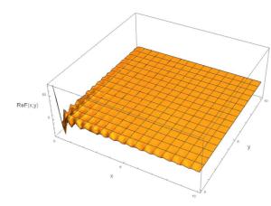
(24) $ \approx F(x) = \int_\epsilon ^K {\rm d} k\frac{{\omega + \mu }}{k}{{\rm e}^{{\rm i}kx}}. $

(25) This is evaluated numerically and shown in Fig. 1.
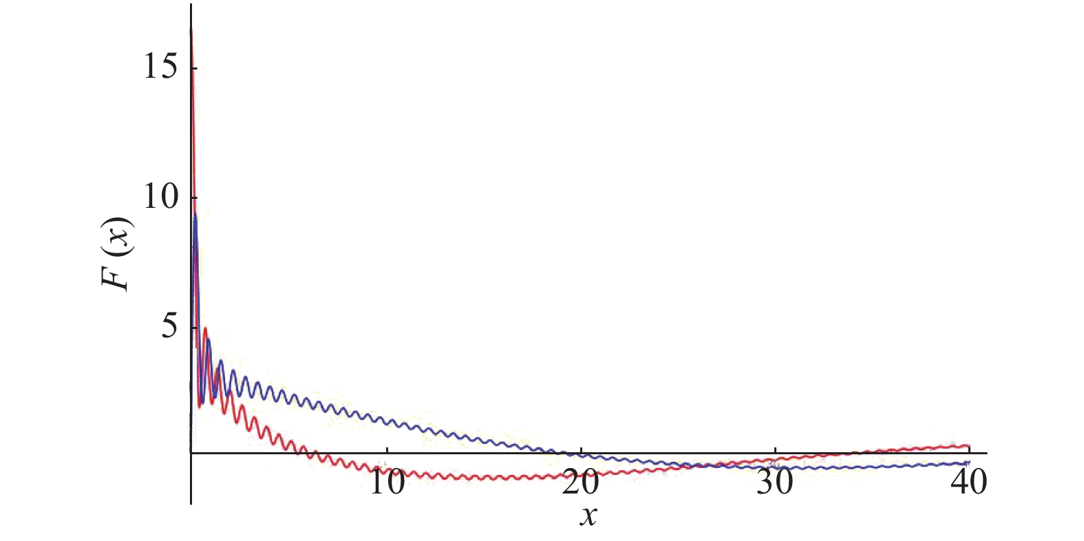
Figure 1. (color online) Red and blue lines represent the real and imaginary part of the integral (25), respectively. Both the real and imaginary parts of the integral decrease quickly with distance, and the long range contribution is very small.
$\epsilon=0.1$ and K = 10 are used in this plot.The figure shows that the interaction between sites falls over large distances. The sites near the boundary make the main contribution to the entanglement entropy.
-
In 2+1 dimensions at t = 0, the Majorana field with
$ \gamma^\mu=(\sigma_y,-i\sigma_z,i\sigma_x) $ has the form [16]$ \begin{split} \psi (\vec x) =& \int {\frac{{{\rm d^2}\vec k}}{{2\pi }}} \frac{1}{{\sqrt {2\omega } }}\left[ {\frac{1}{{\sqrt {\omega + {k_y}} }}\left( {\begin{array}{*{20}{c}} {\omega + {k_y}}\\ {{k_x} + i\mu } \end{array}} \right){b_k}}\right.\\&\left.{ + \frac{1}{{\sqrt {\omega - {k_y}} }}\left( {\begin{array}{*{20}{c}} {\omega - {k_y}}\\ { - {k_x} - i\mu } \end{array}} \right)b_{ - k}^\dagger } \right]{{\rm e}^{{\rm i}\vec k \cdot \vec x}}, \end{split} $

(26) where the annihilation and creation operators bk and
$ b_p^\dagger $ satisfy the anti-commutation relation$ \{b_k,b_p^\dagger\}=\delta(\vec{k}-\vec{p}) $ . We define the vacuum$ |0\rangle $ as the vacuum of this set of operators, i.e.$ b_k|0\rangle=0 $ .Let us consider the following Bogoliubov transformation
$\psi (\vec x) = \int {\frac{{{\rm d^2}\vec k}}{{2\pi }}} \left( {\begin{array}{*{20}{c}} {{a_{1k}}}\\ {{a_{2k}}} \end{array}} \right){{\rm e}^{{\rm i}\vec k \cdot \vec x}},$

(27) which transforms the operators
$ (b_k,b_{-k}^\dagger) $ to the new set of operators$ (a_{1k},a_{2k}) $ . For the 2+1 dimensional Majorana field, we have the relation$\{ {\psi _\alpha }(\vec x),{\psi _\beta }(\vec y)\} = {\delta _{\alpha \beta }}\delta (\vec x - \vec y),$

(28) where
$ \alpha,\beta=0,1 $ represent two components of the Majorana field. To satisfy (28), the operator$ a_{1k} $ and$ a_{2p} $ should have the relation$\{ {a_{ik}},{a_{jp}}\} = {\delta _{ij}}\delta (\vec k + \vec p),$

(29) where
$ i,j=1,2 $ . We choose${a_{1k}} = \frac{1}{{\sqrt 2 }}\left({a_k} + a_{ - k}^\dagger \right),$

(30) ${a_{2k}} = - i\frac{1}{{\sqrt 2 }}\left({a_k} - a_{ - k}^\dagger \right),$

(31) where
$ (a_k,a_{-k}^\dagger) $ are new annihilation and creation operators that satisfy the anti-commutation relation$ \{a_k, a_p^\dagger\}=\delta(\vec{k}-\vec{p}) $ . We can verify that (30) and (31) satisfy the constraint (29). We define the vacuum$ |\Omega\rangle $ , which is annihilated by ak, i.e.$ a_k|\Omega\rangle=0 $ . Hence, we obtain the Bogoliubov transformation between$ (a_k,a_{-k}^\dagger) $ and$ (b_k,b_{-k}^\dagger) $ $\left( {\begin{array}{*{20}{c}} {{b_k}}\\ {b_{ - k}^\dagger } \end{array}} \right) = - \frac{1}{{2\sqrt \omega }}\sqrt {\frac{{{k_x} - i\mu }}{{{k_x} + i\mu }}} \left( {\begin{array}{*{20}{c}} { - \displaystyle\frac{{{k_x} + i\mu }}{{\sqrt {\omega - {k_y}} }} + i\sqrt {\omega - {k_y}} }&{ - \displaystyle\frac{{{k_x} + i\mu }}{{\sqrt {\omega - {k_y}} }} - i\sqrt {\omega - {k_y}} }\\ { - \displaystyle\frac{{{k_x} + i\mu }}{{\sqrt {\omega - {k_y}} }} - i\sqrt {\omega + {k_y}} }&{ - \displaystyle\frac{{{k_x} + i\mu }}{{\sqrt {\omega + {k_y}} }} + i\sqrt {\omega + {k_y}} } \end{array}} \right)\left( {\begin{array}{*{20}{c}} {{a_k}}\\ {a_{ - k}^\dagger } \end{array}} \right).$

(32) Certainly, we have
${b_k} = - \frac{1}{{2\sqrt \omega }}\sqrt {\frac{{{k_x} - i\mu }}{{{k_x} + i\mu }}} \left( {\left( { - \frac{{{k_x} + i\mu }}{{\sqrt {\omega - {k_y}} }} + i\sqrt {\omega - {k_y}} } \right){a_k} - \left( {\frac{{{k_x} + i\mu }}{{\sqrt {\omega - {k_y}} }} + i\sqrt {\omega - {k_y}} } \right)a_{ - k}^\dagger } \right).$

(33) Because we have
$ b_k|0\rangle=0 $ , the new set of operators satisfy$\left( {\left( { - \frac{{{k_x} + i\mu }}{{\sqrt {\omega - {k_y}} }} + i\sqrt {\omega - {k_y}} } \right){a_k} - \left( {\frac{{{k_x} + i\mu }}{{\sqrt {\omega - {k_y}} }} + i\sqrt {\omega - {k_y}} } \right)a_{ - k}^\dagger } \right)|0\rangle = 0.$

(34) The vacuum
$ |0\rangle $ can be expressed as a state constructed from the new set of operators$\begin{array}{*{20}{l}} {\left| 0 \right\rangle }{ = \displaystyle\frac{1}{\gamma }{{\rm e}^{ - \sum\limits_k {{C_k}} a_k^\dagger a_{ - k}^\dagger }}\left| \Omega \right\rangle }\quad\quad\quad\quad\quad\quad \end{array}$

(35) $ = \frac{1}{\gamma }\prod\limits_k {\left( {1 - {C_k}a_k^\dagger a_{ - k}^\dagger } \right)} \left| \Omega \right\rangle ,\;\;$

(36) where
$ \gamma $ is the normalization factor,$ \left| \Omega \right \rangle $ is the vacuum defined by$ a_k \left| \Omega \right \rangle = 0 $ , and the coefficient Ck is fixed by${C_k} = \frac{{{k_x} + i\mu + i\omega - i{p_y}}}{{{k_x} + i\mu - i\omega + i{p_y}}}.$

(37) Following [4], let us consider a system with a finite number of sites. The inverse Fourier transform of the operator ak is
${a_k} = \sum\limits_{\vec N} {{a_{\vec N}}} {{\rm e}^{ -{\rm i}\vec k \cdot \vec N}},$

(38) where
$ \vec{N} $ is the site label. The vacuum$ \left| \Psi \right \rangle\equiv\left| 0 \right \rangle $ of the operator bk can now be written as$\begin{split} \left| \Psi \right\rangle \simeq & \frac{1}{\gamma }\prod\limits_{\vec k} {\left( {1 - \sum\limits_{\vec N,\vec L} {{C_k}} {{\rm e}^{{\rm i}\vec k \cdot (\vec N - \vec L)}}a_{\vec N}^\dagger a_{\vec L}^\dagger } \right)} \left| \Omega \right\rangle \\ \simeq &\frac{1}{\gamma }\left( {1 - \sum\limits_{\vec k} {\sum\limits_{\vec N,\vec L} {{C_k}} } f_{NL}^ka_{\vec N}^\dagger a_{\vec L}^\dagger } \right)\left| \Omega \right\rangle , \end{split}$

(39) where
$ f^k_{NL}={\rm e}^{{\rm i}\vec{k}\cdot(\vec{N}-\vec{L})} $ . For a simplification of notations, we neglect the vector nation and denote$ \vec{n} $ as n. To compute the entanglement entropy, the configuration space is divided into two regions A and$ \bar{A} $ , where the sites in each region are labelled by small letters (n) and small letters with bars ($ \bar{n} $ ), respectively. The region A we choose can be any subregion of the total system. The state$ \left| \Psi \right \rangle $ is$ \begin{split} \left| \Psi \right\rangle \simeq & \frac{1}{\gamma }(1 - \sum\limits_k {\sum\limits_{nl} {{C_k}} } f_{nl}^ka_n^\dagger a_l^\dagger - \sum\limits_k {\sum\limits_{\bar n\bar l} {{C_k}} } f_{\bar n\bar l}^ka_{\bar n}^\dagger a_{\bar l}^\dagger \\&- \frac{1}{2}\sum\limits_k {\sum\limits_{\bar nl} {{C_k}} } \tilde f_{\bar nl}^ka_{\bar n}^\dagger a_l^\dagger )\left| \Omega \right\rangle , \end{split} $

(40) where
$ \tilde{f}^k_{\bar{n}l} = f^k_{\bar{n}l} + f^k_{l\bar{n}} $ .Following the same procedure of the case in 1+1 dimensional Majorana field, we can obtain the reduced density matrix and the second Rényi entropy S2, which have the same form as (18) and (22), respectively. The only difference is the expression of Ck.
In the 2+1 dimensional Majorana fermion case, the coefficients Ck also control the range of the interaction. The factor
$ \sum_k C_k f^k_{nl} $ can be converted to an integral by taking a continuum limit with an IR cut-off$ \epsilon $ and UV cut-off K$\begin{aligned} {{F_{nl}} = \sum\limits_k {{C_k}} f_{nl}^k}{ \simeq \int_\epsilon ^K {\int_\epsilon ^K {\rm d} } {k_x}{\rm d}{k_y}\frac{{{k_x} + i\mu + i\omega - i{k_y}}}{{{k_x} + i\mu - i\omega + i{k_y}}}{{\rm e}^{{\rm i}\vec k \cdot (\vec n - \vec l)a}}} \end{aligned}$

(41) $ \approx F(x,y) = \int_\epsilon ^K {\int_\epsilon ^K {\rm d} } {k_x}{\rm d}{k_y}\frac{{{k_x} + i\mu + i\omega - i{k_y}}}{{{k_x} + i\mu - i\omega + i{k_y}}}{{\rm e}^{{\rm i}({k_x}x + {k_y}y)}}.$

(42) This is evaluated numerically and shown in Fig. 2.

Figure 2. (color online) Plots of integral (42) in 2+1 dimensional Majorana fermion model. The left and right figures represent the real and imaginary parts of the integral, respectively. The amplitude of the surface decreases quickly with distance, and the long range contribution can be neglected.
$\epsilon=0.1$ and K = 10 are used in these plots.The figures show that the interaction between sites diminishes over large distances. The sites near the boundary contribute most significantly to the entanglement entropy. Hence, an area law is expected in this model.
-
In this section, we consider the 2+1 dimensional free U(1) gauge field in the light-cone gauge. To this end, we derive the Lagrangian, and verify that it is the same as a massless scalar field. Subsequently, we perform the Bogoliubov transformation to calculate the entropy.
-
We consider the entanglement entropy of 2+1 dimensional Maxwell fields with light-cone gauge-fixing. In this study, we use the Minkowski metric
$ \eta_{\mu\nu}={\rm diag}(-1,1,1) $ with the Minkowski coordinate$ (x^0,x^1,x^2) $ . We also introduce the light-cone coordinate$ x^+,x^-,x^2 $ with${x^ \pm } \equiv \frac{1}{{\sqrt 2 }}({x^0} \pm {x^1}).$

(43) With regard to the light-cone coordinate, interested readers can read the book [18]. In the light-cone gauge, the vector is defined as
${a^ \pm } \equiv \frac{1}{{\sqrt 2 }}({a^0} \pm {a^1}),$

(44) and the metric becomes
${\hat \eta _{\mu \nu }} = \left( {\begin{array}{*{20}{c}} 0&{ - 1}&0\\ { - 1}&0&0\\ 0&0&1 \end{array}} \right).$

(45) The vector in the light-cone gauge has the properties
$ a_+=-a^- $ and$ a_-=-a^+ $ .Following is the calculation of the 2+1 dimensional Maxwell fields. We start with the Lagrangian
$ \mathcal{L}\!=\!-\!\displaystyle\frac{1}{4}F_{\mu\nu}F^{\mu\nu} $ . Because$ \mathcal{L} $ is a scalar,$ \mu $ ;$ \nu $ can be 0, 1, 2 or +, −, 2. We start with the light-cone coordinate. Because of the asymmetry of$ F_{\mu\nu} $ ,$ F_{++}=F_{--}=F_{22}=0 $ , the Lagrangian becomes${\cal L} = - \frac{1}{4}{F_{\mu \nu }}{F^{\mu \nu }} = - \frac{1}{4}\left( {2{F_{ + - }}{F^{ + - }} + 2{F_{ + 2}}{F^{ + 2}} + 2{F_{ - 2}}{F^{ - 2}}} \right).$

(46) For the light-cone gauge,
$ A^+=0 $ and$ A_-=-A^+=0 $ . By imposing the gauge-fixing, we find that the Lagrangian becomes${\cal L} = \frac{1}{2}{({\partial _ - }{A^ - })^2} + {\partial _ - }{A^2}({\partial _ + }{A^2} + {\partial _2}{A^ - }).$

(47) With the light-cone gauge fixing
$ A^+(p)=0 $ , we have$ A^-=\displaystyle\frac{1}{p^+}(p^2A^2) $ [18]. We perform the Fourier transformation${A^\mu }(x) = \int {\frac{{{\rm d^3}p}}{{{{(2\pi )}^3}}}} {{\rm e}^{{\rm i}px}}{A^\mu }(p).$

(48) The Fourier transformation of
$ \mathcal{L} $ is$\begin{split} \tilde {\cal L} =& - \frac{1}{2}{({p_ - }{A^ - })^2} - {p_ - }{A^2}({p_ + }{A^2} + {p_2}{A^ - })\\ =& - \frac{1}{2}{({p_ - }\frac{1}{{{p^ + }}}{p^2}{A^2})^2} - {p_ - }{A^2}({p_ + }{A^2} + {p_2}\frac{1}{{{p^ + }}}{p^2}{A^2})\\ = & - \frac{1}{2}{({p^2}{A^2})^2} + {p_ - }{A^2}{p^ - }{A^2} + {p_2}{A^2}{p^2}{A^2}\\ = &\frac{1}{2}{({p^2}{A^2})^2} + {p_ - }{A^2}{p^ - }{A^2}. \end{split}$

(49) When written in the momentum space of Minkowski spacetime, it becomes
$\begin{split} \tilde {\cal L} =& \frac{1}{2}{({p^2}{A^2})^2} - \frac{1}{2}({({p^0})^2} - {({p^1})^2}){({A^2})^2}\\ = & - \frac{1}{2}{({p^0}{A^2})^2} + \frac{1}{2}({({p^1}{A^2})^2} + {({p^2}{A^2})^2}). \end{split}$

(50) When we perform the inverse Fourier transformation and return to Minkowski coordinates, the expression becomes
${\cal L} = \frac{1}{2}{({\partial _0}{A^2})^2} - \frac{1}{2}[{({\partial _1}{A^2})^2} + {({\partial _2}{A^2})^2}].$

(51) This is exactly the same Lagrangian as the massless scalar field, and the corresponding Hamiltonian is
${\cal H} = \frac{1}{2}{({\partial _0}{A^2})^2} + \frac{1}{2}[{({\partial _1}{A^2})^2} + {({\partial _2}{A^2})^2}].$

(52) To simplify the notation in the next subsection, we depict
$ A^2 $ as$ A^y $ . The Lagrangian and Hamiltonian can be written as${\cal L} = \frac{1}{2}{({\partial _t}{A^y})^2} - \frac{1}{2}[{({\partial _x}{A^y})^2} + {({\partial _y}{A^y})^2}],$

(53) ${\cal H} = \frac{1}{2}{({\partial _t}{A^y})^2} + \frac{1}{2}[{({\partial _x}{A^y})^2} + {({\partial _y}{A^2})^2}].$

(54) Here, there is no gauge redundancy in the Lagrangian (53). The Hilbert space of
$ A^y $ should have the tensor product structure, so we can consider its entanglement entropy. It behaves like a free scalar field, which coincides with the trivial center case of [11]. -
In the 2+1 dimensional U(1) gauge field with the light-cone gauge, from (53), we have the equation of motion
$\Box {A^y} = 0,$

(55) where
$ \Box=-\displaystyle\frac{\partial^2}{\partial t^2}+\displaystyle\frac{\partial^2}{\partial x^2}+\displaystyle\frac{\partial^2}{\partial y^2} $ . We can find that there is only one physical degree of freedom in the 2+1 dimensional U(1) gauge field, and the component with physical freedom$ A^y $ satisfies the equation for the massless scalar field. For the non-zero components of the gauge field, we have the solution$\left( {\begin{array}{*{20}{c}} {{A^y}}\\ {{{\dot A}^y}} \end{array}} \right) = \int {\frac{{{\rm d^2}\vec k}}{{2\pi }}} \frac{1}{{\sqrt {2\omega } }}\left( {\begin{array}{*{20}{c}} 1\\ { - i\omega } \end{array}} \right){b_k}{{\rm e}^{{\rm i}\vec k \cdot \vec x}} + \left( {\begin{array}{*{20}{c}} 1\\ {i\omega } \end{array}} \right)b_{ - k}^\dagger {{\rm e}^{{\rm i}\vec k \cdot \vec x}}.$

(56) Let us consider a Bogoliubov transformation, which transforms the set of operators
$ (b_k, b_{-k}^\dagger) $ to the following set of operators$\left( {\begin{array}{*{20}{c}} {{A^y}}\\ {{{\dot A}^y}} \end{array}} \right) = \int {\frac{{{\rm d^2}\vec k}}{{2\pi }}} \left( {\begin{array}{*{20}{c}} {{a_{1k}}}\\ {{a_{2k}}} \end{array}} \right){{\rm e}^{{\rm i}\vec k \cdot \vec x}}.$

(57) With operator
$ a_{1k} $ and$ a_{2k} $ , the commutation relations of$ A^{y} $ and$ \dot{A}^y $ are expressed as below$ \begin{split} [{A^y}(\vec x,t),{\dot A^y}(\vec y,t)] =& \int {\frac{{{\rm d^2}\vec k}}{{2\pi }}} \int {\frac{{{\rm d^2}\vec p}}{{2\pi }}} [{a_{1k}},{a_{2p}}]{{\rm e}^{{\rm i}(\vec k \cdot \vec x + \vec p \cdot \vec y)}} \\=& i\delta (\vec x - \vec y), \end{split} $

(58) $[{A^y}(\vec x,t),{A^y}(\vec y,t)] = [{\dot A^y}(\vec x,t),{\dot A^y}(\vec y,t)] = 0.$

(59) We need to have
$[{a_{1k}},{a_{2p}}] = i\delta (\vec k + \vec p),$

(60) $[{a_{1k}},{a_{1p}}] = [{a_{2k}},{a_{2p}}] = 0.$

(61) We choose
${a_{1k}} = \frac{1}{{\sqrt {2\alpha } }}\left({a_k} + a_{ - k}^\dagger \right),$

(62) ${a_{2k}} = - i\sqrt {\frac{\alpha }{2}} \left({a_k} - a_{ - k}^\dagger \right),$

(63) where
$ \alpha $ is a real parameter. The operator ak and$ a_p^\dagger $ have the commutation relations$\left[{a_k},a_p^\dagger \right] = \delta (\vec k - \vec p),$

(64) $[{a_k},{a_p}] = \left[a_k^\dagger ,a_p^\dagger \right] = 0.$

(65) We define
$ a_k|\Omega\rangle=0 $ , where$ |\Omega\rangle $ is the vacuum of the new set of operators. We find that (62) and (63) satisfy (60) and (61). Thus, from (56), (57), (62), and (63), we have the Bogoliubov transformation$\left( {\begin{array}{*{20}{c}} {{b_k}}\\ {b_{ - k}^\dagger } \end{array}} \right) = \frac{1}{{i\sqrt {2\omega } }}\left( {\begin{array}{*{20}{c}} {\displaystyle\frac{{i\omega }}{{\sqrt {2\alpha } }} + i\sqrt {\displaystyle\frac{\alpha }{2}} }&{\displaystyle\frac{{i\omega }}{{\sqrt {2\alpha } }} - i\sqrt {\displaystyle\frac{\alpha }{2}} }\\ {\displaystyle\frac{{i\omega }}{{\sqrt {2\alpha } }} - i\sqrt {\displaystyle\frac{\alpha }{2}} }&{\displaystyle\frac{{i\omega }}{{\sqrt {2\alpha } }} + i\sqrt {\displaystyle\frac{\alpha }{2}} } \end{array}} \right)\left( {\begin{array}{*{20}{c}} {{a_k}}\\ {a_{ - k}^\dagger } \end{array}} \right),$

(66) with
$ \omega=\sqrt{k_x^2+k_y^2} $ . From the above Bogoliubov transformation, we have${b_k} = \frac{1}{{i\sqrt {2\omega } }}\left( {\left( {\frac{{i\omega }}{{\sqrt {2\alpha } }} + i\sqrt {\frac{\alpha }{2}} } \right){a_k} + \left( {\frac{{i\omega }}{{\sqrt {2\alpha } }} - i\sqrt {\frac{\alpha }{2}} } \right)a_{ - k}^\dagger } \right).$

(67) Here
$ (a_k,a_{-k}^\dagger) $ are the annihilation and creation operators of the new modes. We also have the vacuum$ |0\rangle $ , which is annihilated by bk${b_k}|0\rangle = 0.$

(68) From (67), we find that the new set of operators satisfy
$\left( {\left( {\frac{{i\omega }}{{\sqrt {2\alpha } }} + i\sqrt {\frac{\alpha }{2}} } \right){a_k} + \left( {\frac{{i\omega }}{{\sqrt {2\alpha } }} - i\sqrt {\frac{\alpha }{2}} } \right)a_{ - k}^\dagger } \right)|0\rangle = 0.$

(69) The vacuum
$ |0\rangle $ can be expressed in terms of a state constructed from the new set of operators$\begin{array}{*{20}{l}} {\left| 0 \right\rangle }{ = \displaystyle\frac{1}{\gamma }{{\rm e}^{ - \sum\limits_k {{C_k}} a_k^\dagger a_{ - k}^\dagger }}\left| \Omega \right\rangle }\quad\quad\quad\quad\quad\quad \end{array}$

(70) $ \simeq \frac{1}{\gamma }\prod\limits_k {\left( {1 - {C_k}a_k^\dagger a_{ - k}^\dagger } \right)} \left| \Omega \right\rangle ,\;$

(71) where
$ \gamma $ is the normalization factor,$ \left| \Omega \right \rangle $ is the vacuum defined by$ a_k \left| \Omega \right \rangle = 0 $ , and the coefficient Ck is fixed by${C_k} = \frac{{\omega - \alpha }}{{\omega + \alpha }}.$

(72) We find that the Bogoliubov transformation of the light-cone gauge field is very similar to that of the free scalar field [4].
Let us consider a system with a finite number of sites. The inverse Fourier transform of the operator ak is
${a_k} = \sum\limits_{\vec N} {{a_{\vec N}}} {{\rm e}^{ -{\rm i}\vec k \cdot \vec N}},$

(73) where
$ \vec{N} $ is the site label. The vacuum$ \left| \Psi \right \rangle\equiv\left| 0 \right \rangle $ of the operator bk can now be written as$\begin{split} \left| \Psi \right\rangle \simeq & \frac{1}{\gamma }\prod\limits_{\vec k} {\left( {1 - \sum\limits_{\vec N,\vec L} {{C_k}} {{\rm e}^{{\rm i}\vec k \cdot (\vec N - \vec L)}}a_{\vec N}^\dagger a_{\vec L}^\dagger } \right)} \left| \Omega \right\rangle \\ \simeq &\frac{1}{\gamma }\left( {1 - \sum\limits_{\vec k} {\sum\limits_{\vec N,\vec L} {{C_k}} } f_{NL}^ka_{\vec N}^\dagger a_{\vec L}^\dagger } \right)\left| \Omega \right\rangle , \end{split}$

(74) where
$ f^k_{NL}={\rm e}^{{\rm i}\vec{k}\cdot(\vec{N}-\vec{L})} $ . For a simplification of notations, we neglect the vector nation and denote$ \vec{n} $ as n. To compute the entanglement entropy, the configuration space is divided into two regions A and$ \bar{A} $ , where the sites in each region are labelled by small letters (n) and small letters with bars ($ \bar{n} $ ), respectively. The region A can be chosen as any subregion of the total system. The state$ \left| \Psi \right \rangle $ is$ \begin{split} \left| \Psi \right\rangle \simeq & \frac{1}{\gamma }\left(1 - \sum\limits_k {\sum\limits_{nl} {{C_k}} } f_{nl}^ka_n^\dagger a_l^\dagger - \sum\limits_k {\sum\limits_{\bar n\bar l} {{C_k}} } f_{\bar n\bar l}^ka_{\bar n}^\dagger a_{\bar l}^\dagger\right. \\ &\left. - \frac{1}{2}\sum\limits_k {\sum\limits_{\bar nl} {{C_k}} } \tilde f_{\bar nl}^ka_{\bar n}^\dagger a_l^\dagger \right)\left| \Omega \right\rangle , \end{split} $

(75) where
$ \tilde{f}^k_{\bar{n}l} = f^k_{\bar{n}l} + f^k_{l\bar{n}} $ .Following the same procedure of previous cases, we can obtain the reduced density matrix and second Rényi entropy S2, which have the same form as (18) and (22), respectively. The only difference is the expression of Ck.
In 2+1 dimensional U(1) gauge field theory in the light-cone gauge, the coefficients Ck also control the range of the interaction. The factor
$ \sum_k C_k f^k_{nl} $ can be converted to an integral by taking a continuum limit with an IR cut-off$ \epsilon $ and UV cut-off K$\begin{aligned} {{F_{nl}} = \sum\limits_k {{C_k}} f_{nl}^k}{ \simeq \int_\epsilon ^K {\int_\epsilon ^K {\rm d} } {k_x}{\rm d}{k_y}\frac{{\omega - \alpha }}{{\omega + \alpha }}{{\rm e}^{{\rm i}\vec k \cdot (\vec n - \vec l)a}}} \end{aligned}$

(76) $ \approx F(x,y) = \int_\epsilon ^K {\int_\epsilon ^K {\rm d} } {k_x}{\rm d}{k_y}\frac{{\omega - \alpha }}{{\omega + \alpha }}{{\rm e}^{{\rm i}({k_x}x + {k_y}y)}},$

(77) with
$ \omega=\sqrt{k_x^2+k_y^2} $ . This is evaluated numerically and shown in Fig. 3.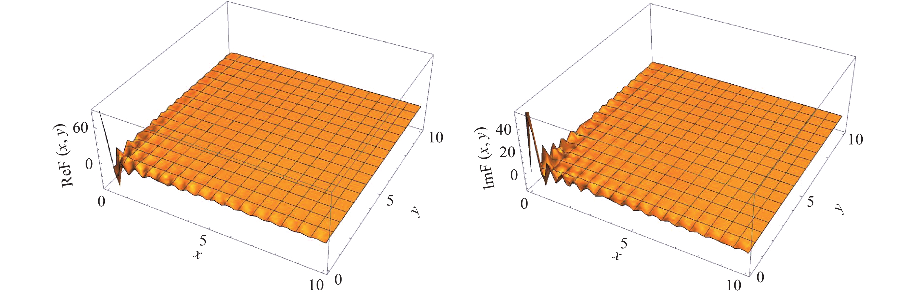
Figure 3. (color online) Plots of integral (77) in 2+1 dimensional U(1) gauge field with light-cone gauge. The left and right figures represent the real and imaginary parts of the integral, respectively. The amplitude of the surface decreases quickly with distance, and the long range contribution can be neglected.
$\epsilon=0.1$ , K = 10 and$\alpha=1$ are used in these plots.The figures show that the interaction between sites diminishes over large distances. The sites near the boundary contribute most significantly to the entanglement entropy. Hence, an area law is expected in this model.
-
In this section, we consider the 3+1 dimensional free spin-2 field theory in the light-cone gauge. To this end, we derive the Lagrangian and find that it is also the same as the massless scalar field. Subsequently, we perform the Bogoliubov transformation to calculate the entropy.
-
We consider the entanglement entropy of the 3+1 dimensional weak gravitational field
$ g_{\mu\nu}=\eta_{\mu\nu}+h_{\mu\nu} $ with light-cone gauge-fixing. Here,$ h_{\mu\nu} $ is a spin-2 field. In this study, we use the Minkowski metric$ \eta_{\mu\nu}={\rm diag}(-1,1,1,1) $ with the Minkowski coordinate$ (x^0,x^1,x^2,x^3) $ . We also introduce the light-cone coordinate$ x^+,x^-,x^2,x^3 $ with${x^ \pm } \equiv \frac{1}{{\sqrt 2 }}({x^0} \pm {x^1}).$

(78) In the light-cone gauge, the vector is defined as
${a^ \pm } \equiv \frac{1}{{\sqrt 2 }}({a^0} \pm {a^1}),$

(79) and the metric becomes
${\hat \eta _{\mu \nu }} = {\hat \eta ^{\mu \nu }} = \left( {\begin{array}{*{20}{c}} 0&{ - 1}&0&0\\ { - 1}&0&0&0\\ 0&0&1&0\\ 0&0&0&1 \end{array}} \right).$

(80) The vector in the light-cone gauge has the properties
$ a_+=-a^- $ and$ a_-=-a^+ $ .Now we come to the calculation of weak gravitational (spin-2) field. We start with the Ricci scalar R. Because R is a scalar,
$ \mu $ ;$ \nu $ can be 0, 1, 2, 3 or +, −, 2, 3. We begin with the light-cone coordinate. We impose the gauge-fixing$ h^{++}=h^{+-}=h^{+I}=0 $ , where$ I=2,3 $ . For the components with subscript indexes, the gauge fixing is$ h_{--}=h_{-+}=h_{-I}=0 $ . For calculating the Ricci scalar R, we use$\Gamma _{\alpha \beta }^\mu = \frac{{{g^{\mu \nu }}}}{2}\left[ {\frac{{\partial {g_{\alpha \nu }}}}{{\partial {x^\beta }}} + \frac{{\partial {g_{\beta \nu }}}}{{\partial {x^\alpha }}} - \frac{{\partial {g_{\alpha \beta }}}}{{\partial {x^\nu }}}} \right]$

(81) and
${R_{\mu \nu }} = {\partial _\alpha }\Gamma _{\mu \nu }^\alpha - {\partial _\nu }\Gamma _{\mu \alpha }^\alpha + \Gamma _{\beta \alpha }^\alpha \Gamma _{\mu \nu }^\beta - \Gamma _{\beta \nu }^\alpha \Gamma _{\mu \alpha }^\beta .$

(82) The Christoffel symbols are
$\Gamma _{ + + }^ + = \frac{1}{2}\frac{{\partial {h_{ + + }}}}{{\partial {x^ - }}},$

(83) $\Gamma _{ + I}^ + = \frac{1}{2}\frac{{\partial {h_{ + I}}}}{{\partial {x^ - }}},$

(84) $\Gamma _{IJ}^ + = \frac{1}{2}\frac{{\partial {h_{IJ}}}}{{\partial {x^ - }}},$

(85) $\Gamma _{ + - }^ + = \Gamma _ {- -} ^ + = \Gamma _{ - I}^ + = 0,$

(86) $\Gamma _{ + + }^ - = - \frac{1}{2}\frac{{\partial {h_{ + + }}}}{{\partial {x^ + }}},$

(87) $\Gamma _{ + - }^ - = - \frac{1}{2}\frac{{\partial {h_{ + + }}}}{{\partial {x^ - }}},$

(88) $\Gamma _ {- -} ^ - = 0,$

(89) $\Gamma _{ + I}^ - = - \frac{1}{2}\frac{{\partial {h_{ + + }}}}{{\partial {x^I}}},$

(90) $\Gamma _{ - I}^ - = - \frac{1}{2}\frac{{\partial {h_{I + }}}}{{\partial {x^ - }}},$

(91) $\Gamma _{IJ}^ - = - \frac{1}{2}\left( {\frac{{\partial {h_{I + }}}}{{\partial {x^J}}} + \frac{{\partial {h_{J + }}}}{{\partial {x^I}}} - \frac{{\partial {h_{IJ}}}}{{\partial {x^ + }}}} \right),$

(92) $\Gamma _{ + + }^I = - \frac{1}{2}\left(2\frac{{\partial {h_{ + I}}}}{{\partial {x^ + }}} - \frac{{\partial {h_{ + + }}}}{{\partial {x^I}}}\right),$

(93) $\Gamma _{ + - }^I = \frac{1}{2}\frac{{\partial {h_{ + I}}}}{{\partial {x^ - }}},$

(94) $\Gamma _ {- -} ^I = 0,$

(95) $\Gamma _{ + J}^I = \frac{1}{2}\left( {\frac{{\partial {h_{ + I}}}}{{\partial {x^J}}} + \frac{{\partial {h_{JI}}}}{{\partial {x^ + }}} - \frac{{\partial {h_{ + J}}}}{{\partial {x^I}}}} \right),$

(96) $\Gamma _{ - J}^I = \frac{1}{2}\frac{{\partial {h_{JI}}}}{{\partial {x^ - }}},$

(97) $\Gamma _{JK}^I = \frac{1}{2}\left( {\frac{{\partial {h_{JI}}}}{{\partial {x^K}}} + \frac{{\partial {h_{KI}}}}{{\partial {x^J}}} - \frac{{\partial {h_{JK}}}}{{\partial {x^I}}}} \right).$

(98) The Ricci scalar is given by
$R = {\hat \eta ^{\mu \nu }}{R_{\mu \nu }} = {\hat \eta ^{ + - }}{R_{ + - }} + {\hat \eta ^{ - + }}{R_{ - + }} + {\hat \eta ^{IJ}}{R_{IJ}} = - 2{R_{ + - }} + {R_{II}},$

(99) where the repeated I, J, and K are summed, and we take this convention below. We have
${R_{ + - }} = - \frac{1}{2}\frac{{{\partial ^2}{h_{ + + }}}}{{\partial {x^{ - 2}}}} + \frac{1}{2}\frac{{{\partial ^2}{h_{ + I}}}}{{\partial {x^I}\partial {x^ - }}} - \frac{1}{4}\frac{{\partial {h_{IJ}}}}{{\partial {x^ - }}}\left( {\frac{{\partial {h_{ + I}}}}{{\partial {x^J}}} + \frac{{\partial {h_{JI}}}}{{\partial {x^ + }}} - \frac{{\partial {h_{ + J}}}}{{\partial {x^I}}}} \right)$

(100) and
$ \setcounter{equation}{101} \begin{split} {R_{II}} =& \frac{{{\partial ^2}{h_{I + }}}}{{\partial {x^ - }\partial {x^I}}} + \frac{{{\partial ^2}{h_{IJ}}}}{{\partial {x^J}\partial {x^I}}} - \frac{1}{2}{\left( {\frac{{\partial {h_{ + I}}}}{{\partial {x^ - }}}} \right)^2} - \frac{{\partial {h_{IJ}}}}{{\partial {x^ - }}}\left( {\frac{{\partial {h_{IJ}}}}{{\partial {x^ + }}} - \frac{{\partial {h_{I + }}}}{{\partial {x^J}}}} \right) \\&- \frac{1}{4}\left[ {{{\left( {\frac{{\partial {h_{JK}}}}{{\partial {x^I}}}} \right)}^2} - {{\left( {\frac{{\partial {h_{IK}}}}{{\partial {x^J}}} - \frac{{\partial {h_{JI}}}}{{\partial {x^K}}}} \right)}^2}} \right].\;\;\;\quad\quad\quad\quad\quad\quad(101) \end{split} $

The Ricci scalar can be written as
$ \setcounter{equation}{102} \begin{split} R =& \frac{{{\partial ^2}{h^{ - - }}}}{{\partial {x^{ - 2}}}} + \frac{{\partial {h^{IJ}}}}{{\partial {x^I}\partial {x^J}}} + \frac{1}{2}\frac{{\partial {h^{IJ}}}}{{\partial {x^ - }}}\left( { - \frac{{\partial {h^{ - I}}}}{{\partial {x^J}}} + \frac{{\partial {h^{JI}}}}{{\partial {x^ + }}} + \frac{{\partial {h^{ - J}}}}{{\partial {x^I}}}} \right)\\ & - \frac{1}{2}{\left( {\frac{{\partial {h^{ - I}}}}{{\partial {x^ - }}}} \right)^2} - \frac{{\partial {h^{IJ}}}}{{\partial {x^ - }}}\left( {\frac{{\partial {h^{IJ}}}}{{\partial {x^ + }}} + \frac{{\partial {h^{I - }}}}{{\partial {x^J}}}} \right) \\&- \frac{1}{4}\left[ {{{\left( {\frac{{\partial {h^{JK}}}}{{\partial {x^I}}}} \right)}^2} - {{\left( {\frac{{\partial {h^{IK}}}}{{\partial {x^J}}} - \frac{{\partial {h^{JI}}}}{{\partial {x^K}}}} \right)}^2}} \right].\quad\;\;\quad\quad\quad\quad\quad\quad(102) \end{split}$

When expressed in Fourier space and considering the light-cone gauge-fixing, we can obtain [18]
${h^{I - }} = \frac{1}{{{p^ + }}}{p_J}{h^{IJ}}$

(103) and
${h^{ - - }} = \frac{1}{{{p^ + }}}{p_I}{h^{ - I}} = \frac{{{p_I}{p_J}}}{{{{({p^ + })}^2}}}{h^{IJ}}.$

(104) With the above relations, we have
$ \begin{split} R =& - 2{p_I}{p_J}{h^{IJ}} + \frac{1}{2}{p_ - }{p_ + }{h^{IJ}}{h^{IJ}} - \frac{1}{2}{p_J}{p_K}{h^{IJ}}{h^{IK}}\\& + \frac{1}{4}\left[{\left({p_I}{h^{JK}}\right)^2} - {\left({p_J}{h^{IK}} - {p_K}{h^{JI}}\right)^2}\right]. \end{split} $

(105) Because
$ h^{IJ} $ is symmetric and traceless, there are only two degrees of freedom$ h^{22} $ and$ h^{23} $ . We expand the above expression with$ I,J,K=2,3 $ , and obtain$\begin{split} R = & - 2{p_I}{p_J}{h^{IJ}} + \left({p_ + }{p_ - } - \frac{1}{2}p_2^2 - \frac{1}{2}p_3^2\right)\left[{\left({h^{22}}\right)^2} + {\left({h^{23}}\right)^2}\right]\\ = & - 2{p_I}{p_J}{h^{IJ}} + \frac{1}{2}\left({\left({p^0}\right)^2} - {\left({p^1}\right)^2} - {\left({p^2}\right)^2} - {\left({p^3}\right)^2}\right)\\&\times\left[{\left({h^{22}}\right)^2} + {\left({h^{23}}\right)^2}\right]. \end{split}$

(106) Apart from the total derivative term
$ \partial_I\partial_J h^{IJ} $ , the Lagrangian of the gravitational field can be written as${\cal L} = \frac{1}{2}\left( {{{({\partial _t}{h^{yy}})}^2} - {{(\nabla {h^{yy}})}^2} + {{({\partial _t}{h^{yz}})}^2} - {{(\nabla {h^{yz}})}^2}} \right),$

(107) where
$ \nabla=\partial_x \vec{i}+\partial_y \vec{j}+\partial_z \vec{k} $ . We have replaced$ h^{22} $ and$ h^{23} $ with$ h^{yy} $ and$ h^{yz} $ respectively.There is no gauge redundancy in the Lagrangian (107). We can expect that the Hilbert space of$ h^{yy} $ and$ h^{yz} $ should have the tensor product structure, so we can consider the entanglement entropy of this model. Hence, we provide a prescription of the entanglement entropy of a free spin-2 field. -
In the 3+1 dimensional gravitational (spin-2) field with the light-cone gauge, we have two independent degrees of freedom. From (107), we have the equations of motion
$\Box {h^{yy}} = 0,\;\Box {h^{yz}} = 0.$

(108) The equations of motion are the same as the free massless scalar field. Their solutions are
${h^{yy}}(x) = \int {\frac{{{\rm d^3}\vec k}}{{\sqrt {2\omega } }}} \left( {{b_k}{{\rm e}^{ -{\rm i}\vec k \cdot \vec x}} + b_k^\dagger {{\rm e}^{{\rm i}\vec k \cdot \vec x}}} \right)$

(109) and
${h^{yz}}(x) = \int {\frac{{{\rm d^3}\vec k}}{{\sqrt {2\omega } }}} \left( {b_k'{{\rm e}^{ -{\rm i}\vec k \cdot \vec x}} + b_k^{'\dagger }{{\rm e}^{{\rm i}\vec k \cdot \vec x}}} \right)$

(110) respectively, where
$ (b_k, b_k^\dagger) $ and$ (b^{'}_k, b_k^{'\dagger}) $ are the creation and annihilation operators of two physical degrees of freedom.Let us consider the mode
$ (b_k, b_k^\dagger) $ . For the operator$ h^{yy} $ , its canonical momentum is$ \dot{h}^{yy} $ . We obtain the solution$\left( {\begin{array}{*{20}{c}} {{h^{yy}}}\\ {{{\dot h}^{yy}}} \end{array}} \right) = \int {\frac{{{\rm d^3}\vec k}}{{{{(2\pi )}^{\frac{3}{2}}}}}} \frac{1}{{\sqrt {2\omega } }}\left( {\begin{array}{*{20}{c}} 1\\ { - i\omega } \end{array}} \right){b_k}{{\rm e}^{{\rm i}\vec k \cdot \vec x}} + \left( {\begin{array}{*{20}{c}} 1\\ {i\omega } \end{array}} \right)b_{ - k}^\dagger {{\rm e}^{{\rm i}\vec k \cdot \vec x}}.$

(111) Let us consider a Bogoliubov transformation, which transforms the set of operators
$ (b_k, b_{-k}^\dagger) $ to the following set of operators$\left( {\begin{array}{*{20}{c}} {{h^{yy}}}\\ {{{\dot h}^{yy}}} \end{array}} \right) = \int {\frac{{{\rm d^3}\vec k}}{{{{(2\pi )}^{\frac{3}{2}}}}}} \left( {\begin{array}{*{20}{c}} {{a_{1k}}}\\ {{a_{2k}}} \end{array}} \right){{\rm e}^{{\rm i}\vec k \cdot \vec x}}.$

(112) With operator
$ a_{1k} $ and$ a_{2k} $ , the commutation relations of$ h^{yy} $ and$ \dot{h}^{yy} $ are expressed as below$\begin{split}[{h^{yy}}(\vec x,t),{\dot h^{yy}}(\vec y,t)] =& \int {\frac{{{\rm d^3}\vec k}}{{{{(2\pi )}^{\frac{3}{2}}}}}} \int {\frac{{{\rm d^3}\vec p}}{{{{(2\pi )}^{\frac{3}{2}}}}}} [{a_{1k}},{a_{2p}}]{{\rm e}^{{\rm i}(\vec k \cdot \vec x + \vec p \cdot \vec y)}}\\ =& i\delta (\vec x - \vec y), \end{split} $

(113) $[{h^{yy}}(\vec x,t),{h^{yy}}(\vec y,t)] = [{\dot h^{yy}}(\vec x,t),{\dot h^{yy}}(\vec y,t)] = 0.$

(114) We find that apart from the dimension, the Bogoliubov 3+1 dimensional spin-2 field with the light-cone gauge is the same as that of the 2+1 dimensional U(1) gauge field. Moreover, they are both the same with the free scalar field. The form of the Bogoliubov transformation is the same as (66), with
$ \omega=\sqrt{k_x^2+k_y^2+k_z^2} $ .We define the vacuum
$ |0\rangle $ by$ b_k|0\rangle=0 $ , and the vacuum$ |\Omega\rangle $ by$ a_k|\Omega\rangle=0 $ in the 3+1 dimensional spin-2 field with the light-cone gauge. Because of the Bogoliubov transformation, the vacuum$ |0\rangle $ can be expressed by the vacuum$ |\Omega\rangle $ and operator$ (a_k,a_p^\dagger) $ as$\begin{aligned} {\left| 0 \right\rangle }{ = \frac{1}{\gamma }{{\rm e}^{ - \sum\limits_k {{C_k}} a_k^\dagger a_{ - k}^\dagger }}\left| \Omega \right\rangle }\quad\quad\quad\quad\quad \end{aligned}$

(115) $ \simeq \frac{1}{\gamma }\prod\limits_k {\left( {1 - {C_k}a_k^\dagger a_{ - k}^\dagger } \right)} \left| \Omega \right\rangle ,\;$

(116) where
$ \gamma $ is the normalization factor, and the coefficient Ck is fixed by${C_k} = \frac{{\omega - \alpha }}{{\omega + \alpha }},$

(117) with
$ \omega=\sqrt{k_x^2+k_y^2+k_z^2} $ .We can consider a system with a finite number of sites. We can divide the system into two parts, A and
$ \bar{A} $ . The region A we choose can be any subregion of the total system. Considering the state$ |\Psi\rangle=|0\rangle $ , we can obtain the reduced density matrix$ \rho_A $ and the second Rényi entropy S2, which have the same form of the cases in previous sections. The only difference is the expression of Ck.In the 3+1 dimensional spin-2 field with the light-cone gauge, the coefficients Ck also control the range of the interaction. The factor
$ \sum_k C_k f^k_{nl} $ can be converted to an integral by taking a continuum limit with an IR cut-off$ \epsilon $ and UV cut-off K$\begin{aligned} {{F_{nl}} = \sum\limits_k {{C_k}} f_{nl}^k}{ \simeq \int_\epsilon ^K {\int_\epsilon ^K {\int_\epsilon ^K {\rm d} } } {k_x}{\rm d}{k_y}{\rm d}{k_z}\frac{{\omega - \alpha }}{{\omega + \alpha }}{{\rm e}^{{\rm i}\vec k \cdot (\vec n - \vec l)a}}} \end{aligned}$

(118) $ \approx F(x,y,z) = \int_\epsilon ^K {\int_\epsilon ^K {\int_\epsilon ^K {\rm d} } } {k_x}{\rm d}{k_y}{\rm d}{k_z}\frac{{\omega - \alpha }}{{\omega + \alpha }}{{\rm e}^{{\rm i}({k_x}x + {k_y}y + {k_z}z)}},$

(119) with
$ \omega=\sqrt{k_x^2+k_y^2+k_z^2} $ . Numerical evaluation in the special case of x = y = z gives the result shown in Fig. 4.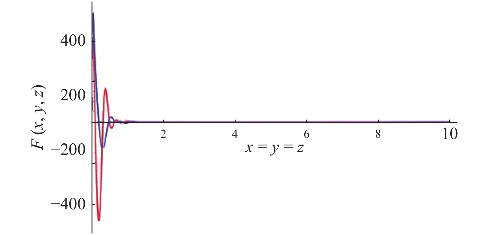
Figure 4. (color online) Plots of integral (119) in 3+1 dimensional gravity with the light-cone gauge in the special case of x = y = z. Both the real and imaginary parts of the integral decrease quickly with distance, and the long range contribution can be neglected.
$\epsilon=0.1$ , K = 10 and$\alpha=1$ are used in this plot.The figure shows that the interaction between sites once again diminishes over large distances. The sites near the boundary contribute most significantly to the entanglement entropy. Hence, an area law is expected in this model as well.
-
In this study, we explore the entanglement of free spin-
$ \displaystyle\frac{1}{2} $ , spin-1 and spin-2 fields. First, we consider the 1+1 dimensional Majorana field, which is just a pair of left and right moving fermions, and the 2+1 dimensional Majorana field. We perform the Bogoliubov transformation of their modes and express the vacuum with a particle pair state in the configuration space. Subsequently, we calculate the second Rényi entropies in the finite systems. Let us emphasize that while a Majorana Weyl fermion is well known to be non-local, a local Hilbert space can be defined when both chiralities are present. This is demonstrated explicitly in the current note. After that, we generalize the method to the 2+1 dimensional free U(1) spin-1 gauge field and the 3+1 dimensional gravitational (free spin-2) field. Because of the gauge redundancy of the higher spin field, there is no Hilbert space with a natural tensor product structure. We take the light-cone gauge for both fields and find that their Lagrangians behave like a free massless scalar field. The light-cone gauge allows simple quantization, while surrendering explicit Lorentz invariance. Nonetheless, it provides a candidate tensor product structure. The definition of entanglement entropy is dependent on both the state and the operator algebra. If the operator algebra is gauge-invariant [10], the corresponding entanglement entropy is likewise gauge-invariant. In this work and in [11], the operator algebras implicitly chosen are not gauge-invariant, such that the corresponding results follow trend. In our past study [11], we explored several different algebras and demonstrated which of those would reproduce the universal log terms found in Casini [10]. It is, however, expected that generic non-gauge invariant algebra choices, such as those considered in the current note, lead to a result that is gauge-dependent. For the U(1) gauge field, the Lagrangian behaves like a scalar field, which coincides with the trivial center case of [11]. As for the gravitational (free spin-2) field, we provide a prescription to observe the tensor product structure of the Hilbert space. Before doing so, there is no prescription of the gravitational (free spin-2) field. After we obtain their Hilbert spaces with a tensor product structure, we calculate the second Rényi entropies. This method can be helpful in dealing with the Hilbert space and entanglement of the perturbative gravitational field, i.e. weak gravitational field. In the non-perturbative regime, the structure of the Hilbert space is still not clear. In all the cases studied, we find that the entropy originates from the particle pairs across the boundary, and the area law emerges naturally.We would like to thank Prof. Yong-Shi Wu for critical and meticulous reading of our manuscript. LYH acknowledges the Thousands Young Talents Program.
Exploring the entanglement of free spin-${\bf\dfrac{1}{2}}$ , spin-1 and spin-2 fields
- Received Date: 2019-01-30
- Available Online: 2019-05-01
Abstract: In this study, we explore the entanglement of free spin-


 DownLoad:
