


 Abstract
 HTML
HTML Reference
 Related
 PDF
PDF


-
What kind of matter can coexist with a black hole in static equilibrium? Evidently, an ordinary matter may not be in equilibrium with a classical black hole because of the gravitational attraction near the horizon and the radiation reaction. Considering quantum mechanical Hawking radiation from the black hole, one may devise an equilibrium system [1]. However, there are well-known examples where matter stays in a stable manner around a black hole, e.g., the charged black hole solution. In the case of the Reissner-Nordström solution, the stress-energy tensor of the electro-magnetic field outside the black hole is anisotropic and satisfies
$ p_1 = -\rho $ in the radial direction and$ p_2 = \rho $ in the transverse direction. Another exact solution was investigated in Ref. [2], in which the matter field is assumed to be isotropic with a negative pressure,$ p = -\rho/3 $ . In this case, the energy density vanishes at the black hole event horizon. Noting these examples, it is worthwhile to analyze the solutions of the Einstein equation with a negative radial pressure and an anisotropic configuration in order to understand the equilibrium configurations of matter and a black hole.A comprehensive collection of static solutions of the Einstein field equation with spherical symmetry can be found in Stephani et. al. [3], Delgaty and Lake [4], and Semiz [5]. Most of them are focused on isotropic fluids because astrophysical observations support isotropy. The perfect Pascalian-fluid (isotropic-fluid) assumption is supported by solid observational and theoretical arguments. The Einstein gravity for such isotropic cases has been studied comprehensively, and hence the recent attention has been drawn by the isotropic objects in new gravity theories such as the massive gravity. In this theory, relativistic stars [6], neutron stars [7], and dyonic black holes [8], for example, have been investigated very recently. Other than this tendency, the anisotropic objects in the Einstein gravity have drawn attention for quite a while. Even though there is no full consensus that anisotropic pressure plays an important role in compact star, interest in anisotropic pressure has grown recently [9-13]. The reader can find other examples related to anisotropic matter in the following works. In relativistic stellar objects, matter with exotic thermodynamical properties that lead to anisotropy was studied in [14, 15] (and references therein). The local anisotropy in self-gravitating systems was studied in [14, 16]. The pressure anisotropy that affects the physical properties such as stability and structure of stellar matter was discussed in [17]. The self-gravitating charged anisotropic fluid with barotropic equation-of-state was considered in [18-20]. For an Einstein-Maxwell system, anisotropic-charged stellar objects consistent with quark stars were studied in Ref. [21]. The Einstein field equation was solved by assuming a specific mass function in Refs. [22-24]. Very recently, the covariant Tolman-Oppenheimer-Volkoff equations for anisotropic fluid were derived in Ref. [25].
Following this recent trend, we consider in this work an anisotropic fluid in order to find exact solutions of the Einstein field equation. Adopting the polar coordinates in
$ S^2 $ , we write the metric for a general spherically symmetric spacetime as (for derivation of field equations, see e.g., Ref. [26])$ {\rm d}s^2 = g_{ab}(x) {\rm d}x^a {\rm d}x^b + r^2(x) ({\rm d}\theta^2 + \sin^2\theta {\rm d}\phi^2), $

(1) where
$ g_{ab} $ is an arbitrary metric in a two-dimensional Lorentzian manifold$ (g_{ab}, M^2) $ . When$ g^{ab} (D_a r) (D_b r) \neq 0 $ , where$ D_a $ is the covariant derivative in$ M^2 $ , we can set$ r $ as a coordinate in$ M^2 $ without loss of generality and then the metric may be written as$ \begin{split}{\rm d}s^2 = & -f(t,r) e^{-\delta(t,r)} {\rm d}t^2 + f(t,r)^{-1} {\rm d}r^2 \\ & + r^2 ({\rm d}\theta^2+ \sin^2\theta {\rm d}\phi^2), \end{split}$

(2) where we do not assume that spacetime is static.
The simplifying assumptions mostly used for matter are those of vacuum, electromagnetic field, and a perfect fluid. For example, the vacuum assumption with ansatz (1) gives uniquely the Schwarzschild metric [27], the simplest and best-known black-hole solution. The stress tensor for an anisotropic fluid compatible with spherical symmetry is
$ T_{\mu\nu} = (\rho+p_2) u_\mu u_\nu + (p_1 - p_2) x_{\mu}x_{\nu} + p_2 g_{\mu\nu}, $

(3) where
$ \rho $ is the energy density measured by an observer comoving with the fluid, and$ u^\mu $ and$ x^\mu $ are its timelike four-velocity and a spacelike unit vector orthogonal to$ u^\mu $ and angular directions, respectively. This$ T_{\mu\nu} $ together with ansatz (1) can describe, for example, the interior of static, spherically symmetric, and extremely high-density stars. In addition, we need to introduce the equation-of-state, which is the relation between$ p_i $ and$ \rho $ . In cosmology, one usually assumes the barotropic condition for the equation-of-state,$ p_i = w_i \rho, $

(4) with
$ w_i=0 $ describing the dust,$ w_i=1/3 $ the radiation,$ w_i < -1/3 $ the dark energy, and$ w_i < -1 $ the phantom energy. Because the energy-momentum tensor is given by$ T^{\nu}_{\mu}= \mbox{diag}(-\rho, p_1,p_2,p_2) $ , one of the Einstein equations$ G^0_1=0 $ gives$ f(r,t) = f(r). $

(5) Several general requirements for
$ T_{\mu\nu} $ are imposed, collectively known as energy conditions. For example, the weak energy condition states that the energy density should be non-negative to every observer. Alternatively, one might impose strong or dominant energy conditions. For the anisotropic fluid, the energy conditions take the following form: the weak energy condition,$ \rho \geqslant 0 $ ,$ \rho + p_i \geqslant 0 $ ; the strong energy condition,$ \rho+p_i \geqslant 0 $ ,$ \rho + \sum_i p_i \geqslant 0 $ ; the dominant energy condition,$ \rho \geqslant |p_i| $ ; and the null energy condition,$ \rho + p_i \geqslant 0 $ .In general,
$ u_\mu $ and$ x_\mu $ can be chosen to be arbitrary timelike and spacelike four-vectors. Since we are trying to find static solutions, we restrict them in the present work to satisfy$ u_\mu \propto (\partial_t)_\mu $ and$ x_\mu \propto (\partial_r)_\mu $ . Let us now consider a matter field across an event horizon described by the fluid form in Eq. (3). Inside the horizon, where$ g_{tt}>0 $ and$ g_{rr} < 0 $ , the coordinate$ r $ plays the role of time. Then$ -p_1 $ and$ -\rho $ play the roles of energy density and pressure along the spatial$ t $ direction, respectively. With this exchange of roles, the energy conditions mentioned above do not change and the energy density and pressure are continuous across the horizon when$ w_1 = -1 $ . In the case of$ w_1 \neq -1 $ , the pressure must be discontinuous at the horizon$ r_H $ unless$ \rho(r_H) =0 $ , which implies that solutions satisfying$ w_1\neq -1 $ and$ \rho(r_H) \neq 0 $ must be dynamical. In this work, we require$ w_1 = -1 $ so that the energy density is continuous across the horizon, which replaces a boundary condition. In Ref. [4], various tests of acceptability for the isotropic fluid, such as the positivity of energy density and pressure, the regularity at the origin, the subluminal sound speed, etc. were applied to a vast number of candidate solutions.Let us describe the motivation for anisotropic matter. The anisotropic fluid can be used to study effectively static matter fields. Traversable wormholes were widely studied recently [28, 29] based on various gravity theories. The solutions require the existence of exotic materials which violate energy conditions and have (effective) negative anisotropic pressures. For example, the Morris-Thorne type wormhole satisfies
$ \rho+ p_1 + 2p_2 =0 $ [30]. As will be shown below, these materials can also be used to support matter outside the black-hole horizon. In the case of a scalar field, the equation-of-state varies depending on the kinetic term. It takes a negative value when the field is non-dynamical, which can be studied by an anisotropic fluid with negative pressure. One example is the monopole-black hole in the nonlinear sigma model, which will be shown later. In the case of a static electric field, the equation-of-state is given by$ p_1 = -\rho $ and$ p_2 = \rho $ , and the trace of the stress-tensor vanishes. This results in the well-known Reissner-Nordström black hole. As was discussed earlier, the condition that matter stays static at the horizon requires$ w_1 = -1 $ explicitly. Therefore, it is worthwhile to study the solutions of the Einstein equation for anisotropic fluid with$ w_1 = -1 $ and various values of$ w_2 $ , as an extension of the Reissner-Nordström black hole.In this work, we consider the case when
$ w_1=-1 $ for which exact analytic solutions exist. We classify the solutions according to the value of$ w_2 $ . In Section 2, we derive the Tolman-Oppenheimer-Volkoff equation for the anisotropic fluid. In Section 3, we obtain the exact solutions for the case$ w_1 = -1 $ . In Section 4, we classify the solutions into six types and discuss the corresponding black-holes. In Section 5, we study the stability of the solutions. We summarize the results in Section 6. -
With the metric (2) and
$ f(t,r) = f(r) $ as in Eq. (5) , and the energy-momentum tensor (3), the Einstein equation becomes$ G^0_0 = -\frac1{r^2} + \frac{f}{r^2} + \frac{f'}{r} = - 8\pi \rho(r), $

(6) $ G^1_1 = -\frac1{r^2} + \frac{f}{r^2}+ \frac{f'}{r} - \frac{f \delta'(t,r)}{r}= 8 \pi p_1(r) , $

(7) $ \begin{split} G^2_2 = & \frac{f'}{r} + \frac{f''}{2} - \frac{f}{2r} \delta'(t,r) -\frac{3f'}{4} \delta '(t,r) +\frac{f}{4} \delta'(t,r)^2 \\ &- \frac{f}2 \delta''(t,r) = 8\pi p_2(r). \end{split}$

(8) Since we assume
$ w_1 = -1 $ , the combination$ G_{0}^{0}- G_{1}^1=0 $ gives$ \delta(t,r) = \delta (t) $ . Redefining the time coordinate, we can set$ \delta =0 $ without loss of generality. The metric now reduces to$ {\rm d}s^2 = - f(r) {\rm d}t^2 + f(r)^{-1} {\rm d}r^2 + r^2 ({\rm d}\theta^2+ \sin^2\theta {\rm d}\phi^2). $

(9) This means that a hypersurface-orthogonal Killing vector exists in spacetime. Thus, spacetime is static in the region where
$ f>0 $ , and$ \rho=\rho(r) $ , and$ p_2 = p_2(r) $ holds for consistency. The first equation (6) can be formally integrated to give$ f(r) = 1-\frac{2m(r)}{r} , $

(10) where the mass function
$ m(r) $ is defined by$ m(r) = 4\pi \int^r r'^2 \rho(r') {\rm d}r'. $

(11) Here, the integration constant is absorbed into the definition of
$ m(r) $ . If one requires the analyticity of spacetime at the center, this requires$ m(r) \simeq m_3 r^3 + m_5 r^5 + \cdots $ around$ r=0 $ , where$ m_3 $ ,$ m_5 $ are constants, which restricts the form of$ \rho(r) $ . Substituting Eq. (10) into Eq. (8), we obtain the expression for$ p_2 $ in terms of$ \rho $ as$ p_2 = -\rho - \frac{r\rho'}{2}, $

(12) which can also be obtained from the conservation law
$ \nabla^\mu T_{\mu \nu} =0 $ . -
The purpose of this work is to find analytic solutions of the Einstein equation. We restrict our interest to the exactly solvable case with
$ w_1=-1. $

(13) When
$ \rho $ has the role of energy density, the energy conditions restrict the types of matter to physically allowed ones. Among these conditions, the positivity of energy density appears to be crucial. In addition, all energy conditions require$ w_2 \geqslant -1 $ . Specifically, the dominant energy condition requires$ w_2 \leqslant 1 $ and the strong energy condition requires$ w_2 \geqslant 0 $ . Therefore, when$0\leqslant $ $ w_2 \leqslant 1 $ , all energy conditions are satisfied. As we assume$ p_2 = w_2 \rho $ , Eq. (12) can be solved to give$ m(r) $ for$ w_2 \neq 1/2 $ , the density and radial pressure$ m(r) = M + \frac{K}{2 r^{2w_2-1}} , \;\; \rho (r) = -p_1(r) = \frac{(1-2w_2) K}{8\pi r^{2+ 2w_2}} , $

(14) where
$ M $ and$ K $ are constants. For energy density to be non-negative, we require$ r_0^{2w_2} \equiv (1-2w_2) K \geqslant 0, $

(15) where the positive parameter
$ r_0 $ for the length (mass) scale was introduced for convenience because the dimension of parameter$ K $ is dependent of the value of$ w_2 $ . The energy density and pressure are singular at the origin or at infinity when$ w_2> -1 $ and$ w_2 < -1 $ , respectively. In order to have a smooth limit$ w_2 \to 1/2 $ , we introduce a new mass parameter$ M' \equiv M + \frac{r_0}{2(1-2w_2)}. $

(16) The solutions for
$ w_2 = 1/2 $ can then be obtained by taking the limit$ w_2\to 1/2 $ of Eq. (14), which gives$ m(r) = M' + \frac{r_0}{2} \log \frac{r}{r_0} , \;\; \rho(r) = \frac{r_0}{8\pi r^3}. $

All other physical formulae for
$ w_2=1/2 $ can be obtained in the same manner. Therefore, we will not discuss the$ w_2=1/2 $ case separately. The metric function in Eq. (10) becomes$ f(r) = 1- \frac{2M}{r} -\frac{K}{r^{2w_2}}, $

(17) where
$ M $ and$ K $ can be rewritten using Eqs. (15) and (16). As we are interested in the solutions with matter, we restrict our interest to the case with$ r_0 \neq 0 $ . For$ 1/2 < w_2 \leqslant 1 $ , the spacetime structure must be very similar to the Reissner-Nordström geometry. For the isotropic fluid with$ w_1=w_2=-1 $ ,$ M $ and$ 3K $ represent the mass of the (anti)-de Sitter black hole and the cosmological constant, respectively. Let us now analyze the curvature singularities. The scalar curvature,$ R = \frac{ w_2-1 }{r_0^2} \left(\frac{r_0}{r}\right)^{2 (w_2+1)}, $

is singular at the origin and at infinity when
$ -1 < w_2 \neq 1 $ and$ w_2 < -1 $ , respectively. Therefore, it is regular everywhere only when$ w_2=-1 $ or 1. The Krestchmann invariant is given by$ \begin{split} R_{abcd}R^{abcd} = & \frac{48 M^2}{ r^{6}}+\frac{16 (w_2+1) (2 w_2+1) M r_0^{2w_2}}{ (1-2w_2) r^{2 w_2+5}}\\ & + \frac{4\left(4w_2^4 + 4w_2^3 + 5w_2^2 +1\right)r_0^{4w_2} }{(1-2w_2)^2 r^{4w_2+ 4} }. \end{split}$

Note that the numerator of the last term is positive definite and the apparent divergence for
$ w_2 = 1/2 $ disappears when the parametrization of Eq. (16) is introduced. Therefore, the term is singular at the origin or at infinity when$ w_2 > -1 $ or$ w_2 < -1 $ , respectively. When$ w_2 = -1 $ , the first term becomes singular at the origin unless$ M= 0 $ . For$ r_0 \neq 0 $ , the Krestchmann invariant is regular everywhere only when$ M=0 $ and$ w_2 =-1 $ , which is nothing else but the (anti)-de Sitter spacetime. In summary, spacetime is singular at infinity when$ w_2 < -1 $ and singular at the origin when$ M \neq 0 $ . The singularities can be naked or covered by (cosmological) event horizons depending on the nature of spacetime.Before discussing the details of each solution, we would like to discuss the positivity of energy density when there exists an event horizon in the solution. Because
$ t $ and$ r $ coordinates exchange their roles of time and space,$ -p_1 $ plays the role of energy density in the region of$ f(r) < 0 $ . Therefore, in the presence of a horizon, the energy density is positive definite over the whole space when$ w_1 < 0 $ and$ \rho>0 $ , which is satisfied by the present solution. -
The properties of the solution of Eq. (17) is completely determined by the functional behavior of
$ f(r) $ . We classify the solutions into six types as following.(I) Schwarzschild:
$ f(r) $ changes the signature from negative to positive with$ r $ .(II) Schwarzschild-de Sitter:
$ f(r) $ changes the signature from negative to positive and then to negative again.(III) Reissner-Nordström:
$ f(r) $ changes the signature from positive to negative and then to positive again.(IV) de Sitter:
$ f(r) $ changes the signature from positive to negative.(V) Naked singular:
$ f(r) $ is positive definite.(VI) Anisotropic cosmological:
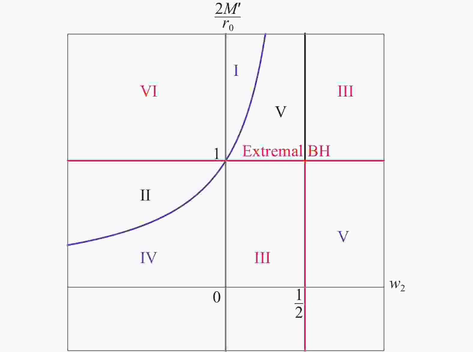
$ f(r) $ is negative definite.The classification of the solutions is shown in Fig. 1. The Roman numbers I-VI denote the type of solution with respect to the value of
$ (w_2, 2M'/r_0) $ .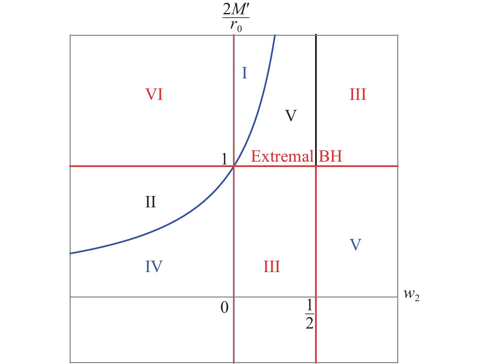
Figure 1. (color online) The classification of the solutions. The horizontal and vertical axes denote
${w_2}$ and${2M'/r_0}$ , respectively. The blue curve represents${2M'/r_0 = (1-2w_2)^{-1}}$ , for which${M=0}$ . Each line in the figure is labeled by the text of the same color.Rather than discuss all the details, let us illustrate only the case of
$ w_2> 1/2 $ . Asymptotically,$ \lim_{r\to \infty} f(r) \to 1 $ . Around the origin,$ f(r) $ is a decreasing function with$ f(0) = \infty $ . Its derivative is$ f'(r) = \frac{2r_0}{r^2}\left[\frac{M}{r_0} - \frac{w_2}{2w_2-1}\left(\frac{r_0}{r} \right)^{2w_2 -1}\right]. $

When
$ M $ is positive,$ f'(r) $ vanishes at$ r_m = [ w_2 r_0/(2w_2- $ $1)M ]^{1/(2w_2-1)} r_0$ and$ f(r) $ has a minimum value at$ r_m $ ,$ \begin{aligned} f(r_m) & = 1- \frac{2M}{r_m} + \frac{1}{2w_2-1} \frac{r_0^{2w_2}}{r_m^{2w_2}} = 1- \left[\frac{(2w_2-1)M}{w_2 r_0}\right]^{2w_2/(2w_2-1)} \\ & = \frac{2w_2-1}{2w_2} \left(1-\frac{2M'}{r_0}\right) \times P, \end{aligned}$

where
$ P $ represents a series function of$ (2w_2-1)M/w_2 r_0 $ , which is positive. The minimum value$ f(r_m) $ is positive when$ 2M'/r_0 < 1 $ . In this case, the metric function is positive definite for all$ r $ and the singularity at the origin is naked. The metric belongs to type V. The case$ M < 0 $ also belongs to this type. On the other hand, when$ f(r_m) < 0 $ i.e.$ 2M'/r_0>1 $ , the spacetime has two horizons at radii$ r_\pm $ satisfying$ f(r_\pm)=0 $ . Therefore, the spacetime is of type III. When$ 2M'/r_0 =1 $ , the two horizons coincide and are extremal.The solutions corresponding to a black hole are of type I, II, and III. Type IV solution is similar to the de Sitter spacetime having a cosmological horizon. On the other hand, type V solution possesses a naked singularity. Type VI solution corresponds to a cosmological solution undergoing anisotropic expansion/contraction, which is bounded by a cosmological horizon. In this case, the singularity at
$ r=0 $ is located at the future/past infinity . -
Type I solutions exist only when
$ 0\leqslant w_2 < 1/2 $ and$ M > 0 $ . The geometry takes the form of a modified Schwarzschild spacetime. The functional form of$ f(r) $ at$ r\simeq 0 $ is governed by the$ -2M/r $ term, which implies that$ r=0 $ is a singularity. The geometry is asymptotically flat because$ f(r) $ approaches a constant value as$ r\to \infty $ . There exists an event horizon$ r_{\rm BH} $ satisfying$ f(r_{\rm BH})=0 $ . However, the energy density is not sufficiently localized so that the total mass diverges as$ r\to \infty. $ If
$ w_2=0 $ , the solution takes a modified Schwarzschild form with a solid angle deficit. After introducing new coordinates$ y = r/\alpha $ and$ \tau = \alpha t $ , where$ \alpha = \sqrt{1- K } $ , the metric becomes$ {\rm d}s^2 = - \left(1- \frac{2\tilde{M}}{y} \right) {\rm d}\tau^2 + \frac{{\rm d}y^2}{1- 2\tilde{M}/y} + (\alpha y)^2 ({\rm d}\theta^2 + \sin^2\theta {\rm d}\phi^2) , $

where
$ \tilde{M} = M/\alpha^3 $ . The horizon is at$ r= 2M/\alpha^2 $ . The mass function increases with$ r $ as$ m(r) = M+ K r/2 $ . At the horizon, it is$ m(r_{\rm BH}) = M/\alpha^2 $ . The fluid with$ w_2=0 $ is equivalent to the self-gravitating global monopole [31], and the monopole-black hole in the nonlinear sigma model with the hedgehog ansatz [32].Type II solution exists only for
$ w_2 < 0 $ with$ (1-2w_2)^{-1} < 2M'/r_0 < 1 $ . The geometry takes the form of the modified Schwarzschild-de Sitter solution. The functional form of$ f(r) $ at$ r\sim 0 $ is governed by the$ -2M/r $ term, which implies that$ r=0 $ is a singularity. Asymptotically,$ f(r) \to - K r^{2|w_2|} $ goes to negative infinity. There are two horizons satisfying$ f(r) =0 $ , one is the black-hole horizon$ r_{-} $ and the other the cosmological horizon$ r_+ $ . The cosmological horizon resembles that of the de Sitter spacetime. When$ w_2 = -1 $ , the geometry becomes the Schwarzschild-de Sitter spacetime with$f(r) = 1-2M/r - $ $K r^2$ .The mass inside
$ r $ monotonically increases. The total mass inside the cosmological horizon becomes$ m(r_+) =\frac{r_+}2\left[\frac{2 M}{r_+} + \frac{1}{1-2w_2} \left(\frac{r_0}{r_+}\right)^{2w_2} \right] = \frac{r_+}2. $

-
Type III is the most interesting because it contains the Reissner-Nordström solution as a specific case with charge
$ Q = r_0 $ when$ w_2 =1 $ . The solution exists when$ 2M'/r_0 \leqslant 1 $ and$ 2M'/r_0 \geqslant 1 $ for$ 0 < w_2 \leqslant 1/2 $ and$ w_2 > 1/2 $ , respectively. The geometry of the type III solution takes the form of the Reissner-Nordström solution in the sense that it has an inner horizon$ r_- $ in addition to the outer black-hole horizon at$ r_{+} $ , given by$ f(r_{+}) =0 $ . For$ w_2 \leqslant 1/2 $ , the mass function increases with$ r $ . Therefore, the solution fails to describe a localized object such as a star.On the other hand, the matter distribution is localized sufficiently if
$ w_2 > 1/2 $ . The total mass over the whole spacetime is finite and is given by$ M = M' + \frac{r_0}{2(2w_2-1)} \geqslant M'. $

(18) Note that
$ f(r_0) = 1- 2M'/r_0 < 0 $ , which implies that$ r_0 $ is located in between the two horizons,$ r_- < r_0 < r_+ $ . The surface gravity of the black hole at$ r= r_+ $ is$ \begin{split} {\kappa} & = \frac{f'(r_+) }2 = \frac{1}{r_+} \left[w_2 - \frac{(2w_2-1)M}{r_+} \right] \\ & = \frac{1}{2r_+} \left[1- \left(\frac{r_0}{r_+}\right)^{2w_2} \right] \geqslant 0. \end{split}$

(19) The entropy and the black hole temperature are given by
$ S = \pi r_+^2, \;\; T_H = \frac{\kappa}{2\pi} = \frac{1}{4\pi r_+} \left[1- \left(\frac{r_0}{r_+}\right)^{2w_2} \right]. $

(20) Treating
$ r_+ $ as a function of$ M $ and$ r_0 $ in the variational relation$ \delta f(r_+) =0 $ in Eq. (17), and using Eqs. (18), (20), one gets the first law of the black hole thermodynamics in the form,$ T_H {\rm d}S = 2\pi T_H r_+ {\rm d}r_+ = \delta M - \Phi \delta r_0 , $

(21) where the potential takes the form,
$ \Phi = \frac{w_2 }{2w_2-1} \left(\frac{r_0}{r_+}\right)^{2w_2-1} . $

(22) For the case
$ w_2 = 1 $ , this provides the correct value of the electric potential with a charge$ Q= r_0 $ . -
Let us check the stability of the spacetime with anisotropic fluid by introducing linear spherical scalar perturbations. Let us write the metric in the form,
$ {\rm d}s^2 = - e^\nu {\rm d}t^2 + e^\lambda {\rm d}r^2 +e^\mu {\rm d}\Omega_2^2. $

(23) The general energy-momentum tensor is given by Eq. (3) with
$ p_i = w_i\rho $ , where the velocity and the radial four-vectors are given by$ \begin{split}& u^\mu = [e^{-\nu/2} \sqrt{1+v^2}, e^{-\lambda/2} v,0,0], \\ & x^\nu = [ e^{-\nu/2} v, e^{-\lambda/2} \sqrt{1+ v^2}, 0,0 ],\end{split}$

(24) where
$ v $ corresponds to a normalized radial velocity and$ x^a u_a = 0 $ . The components of the stress tensor now become$ \begin{split} & T^0_1 = (1+w_1) \rho e^{(\lambda-\nu)/2} v\sqrt{1+v^2}, \\ & T^0_0 = - \rho \big[1+(1+w_1) v^2 \big], \\ & T^1_1 = \rho[w_1+ (1+ w_1) v^2], \\ & T^2_2 = \rho w_2. \end{split}$

(25) We introduce the perturbations of the metric for a given background solution
$ \nu_0(r) $ ,$ \lambda_0(r) $ , and$ \mu_0(r) $ as$ \begin{split} & e^\nu = e^{\nu_0(r)}(1 + \delta \nu), \\ & e^\lambda = e^{\lambda_0(r)}(1 + \delta \lambda), \\ & e^\mu = e^{\mu_0(r)}(1 + \delta \mu) , \\ & \rho = \rho_0 + \delta \rho . \end{split}$

(26) The linearized coordinate transformations of
$ t $ and$ r $ are given by$ t = \tilde t + \delta t(\tilde t, \tilde r),\;\; r = \tilde r + \delta r(\tilde t, \tilde r). $

(27) Under this transformation, the metric (23) can be written as
$ \begin{split} {\rm d}s^2 & = - e^{\nu_0(r)} (1+ \delta \nu ){\rm d} t^2 + e^{\lambda_0(r)} (1+ \delta \lambda) {\rm d} r^2 + e^{\mu_0(r)} (1+ \delta \mu) {\rm d}\Omega^2 \\ & = - e^{\nu_0(\tilde r)} [1+\delta \nu+ \nu_0' \delta r+ \dot \nu_0 \delta t+ 2\dot{\delta t} ]{\rm d}\tilde t^2 \\ & \;\;\; + 2[ e^{\lambda_0} \dot{\delta r} - e^{\nu_0} \delta t'] {\rm d}\tilde t {\rm d} \tilde r \\ & \;\;\; + e^{\lambda_0(\tilde r)} [1+ \delta \lambda + \lambda_0' \delta r + \dot{\lambda}_0 \delta t+ 2\delta r'] {\rm d}\tilde r^2 \\ & \;\;\; + e^{\mu_0(\tilde r)} \left[1+\delta \mu + \mu'_0 \delta r + \dot \mu_0 \delta t\right] {\rm d}\Omega^2 , \quad\quad\quad\quad\quad\quad\quad(28) \end{split} $

where the overdot and the prime denote the derivatives with respect to
$ \tilde t $ and$ \tilde r $ , respectively. In Eq. (28), we can impose$ \dot \nu_0 =0 $ ,$ \dot \lambda_0 =0 $ , and$ \dot \mu_0 =0 $ .We choose the gauge for
$ \delta r $ and$ \delta t $ such that$ \tilde g_{0i}=0 \Rightarrow e^{\lambda_0} \dot \delta r = e^{\nu_0} \delta t', \;\; \delta \tilde \mu \equiv \delta \mu + \mu'_0 \delta r=0 . $

(29) Omitting tilde in
$ \tilde r $ and$ \tilde t $ , the metric (28) becomes$ {\rm d}s^2 \!=\! - e^{\nu_0} [1\!+\! \delta \nu(t,r) ]{\rm d} t^2 \!+\! e^{\lambda_0} [1\!+\! \delta \lambda(t,r)] {\rm d} r^2 \!+\! e^{\mu_0} {\rm d}\Omega^2 . $

(30) The
$ \delta G^0_1 $ part of the Einstein equation based on the metric (30), after introducing$ e^{\nu_0} = f(r) = e^{-\lambda_0} $ , gives$ v $ as$ -\frac{\mu_0' \dot {\delta \lambda}}{2 f(r)} = 8\pi (1+ w_1) \frac{\rho_0 v}{f} \Rightarrow v = - \frac{\mu_0' \dot {\delta \lambda}}{16\pi(1+w_1) \rho_0}. $

(31) We may use this equation as a definition of
$ v $ . The$ \delta G^0_0 $ part,$ -\frac{f(r)}{4} \left[2\mu_0'\delta\lambda' + \left( 4\mu_0'' + 3\mu_0'^2 + \frac{2\mu_0' f'(r)}{f(r)}\right)\delta \lambda \right] = -8\pi \delta \rho, $

(32) provides the definition of
$ \delta \rho $ . The$ \delta G^1_1 $ part becomes$ \frac{f(r)}{4} \left[2 \mu_0'\delta\nu' -\left(\mu_0'^2+ \frac{2\mu_0'f'(r)}{f(r)}\right) \delta \lambda \right] = 8\pi w_1 \delta \rho. $

(33) Combining Eq. (32) and Eq. (33), we write
$ \delta \nu' $ by means of$ \delta \lambda $ and$ \delta \lambda' $ :$ \delta \nu' = w_1 \delta \lambda'+\left[2w_1 \frac{\mu_0''}{\mu_0'}+\frac{1+ 3w_1}{2}\mu_0' +(1+w_1) \frac{f'(r)}{f(r)}\right] \delta \lambda . $

(34) Finally, the
$ \delta G^2_2 $ part becomes$ \begin{split} & -\frac{\ddot {\delta \lambda}}{2f(r)} + \frac{f(r)}{4} \left[ 2 \delta \nu'' + \left( \mu_0'+ \frac{3f'}{f}\right) \delta\nu'- \left(\mu_0'+ \frac{f'}{f}\right)\delta \lambda' \right. \\ & \left.- \left(2\mu_0''+ \mu_0'^2 +\frac{2f''}{f} +\frac{2f'\mu_0'}{f} \right) \delta \lambda \right] = 8\pi w_2 \delta \rho. \end{split}$

(35) Using
$ \mu_0(r) = 2\log r $ after substituting Eqs. (34) and (33) into Eq. (35), we get a differential equation for the perturbation$ \delta \lambda $ $ \begin{split}\frac{\ddot{\delta \lambda}}{f^2(r)} = & w_1 \delta \lambda'' + \left[\frac{2(w_1-w_2)}{r} + \frac{1+ 5w_1}2 \frac{f'(r)}{f(r)}\right]\delta \lambda' + V(r) \delta \lambda, \end{split}$

(36) where
$ \begin{split}V(r) = & - \frac{2w_2}{r^2} + \frac{1+ 5w_1- 4w_2}2 \frac{f'(r)}{rf(r)} \\ & + \frac{1+w_1}2\frac{f'(r)^2}{f(r)^2} +w_1\frac{f''(r)}{f(r)}. \end{split}$

(37) Introducing a new coordinate
$ z $ as$ {\rm d}z = f^{-1} {\rm d}r $ and setting$ \delta \lambda = {\rm e}^{-{\rm i} \omega t} g_1(r) $ , the perturbation equation becomes$ \begin{split}-\frac{{\rm d}^2 g_1}{{\rm d}z^2} & + \left[\frac{2(w_1-w_2)}{w_1 r}f(r) + \frac{1+ 3w_1}{2w_1} f'(r)\right] \frac{{\rm d}g_1}{{\rm d}z} \\ & +V(z) g_1 = \frac{\omega^2}{w_1} g_1, \end{split}$

(38) where
$ V(z) = V(r(z)) $ . For large$ \omega^2 $ , the equation takes the form,$ {\rm d}^2g_1/{\rm d}z^2 \approx (-w_1^{-1}) \omega^2 g_1 $ . Therefore, the system is possibly stable only when$ w_1 \geqslant 0 $ .An interesting situation is the present case with
$ w_1 = -1 $ . The off-diagonal component of the stress tensor$ T_1^0 $ in Eq. (25) vanishes, and from Eq. (31),$ \delta \lambda $ is independent of time ,$ \dot{\delta\lambda} = \ddot{\delta\lambda} =0. $

(39) Eq. (36) then becomes, after introducing
$ \Delta = f \delta \lambda $ ,$ \begin{split} \Delta '' & + \frac{2(1+w_2)}{r} \Delta' + \frac{2w_2}{r^2} \Delta \\ & - (1+w_1) \left[ \Delta'' + \left(\frac{f'}{2f}+ \frac2r\right) \Delta' + \frac{f'}{2rf} \Delta\right] =0 . \end{split} $

(40) For
$ w_1 =-1 $ , and ignoring the term in the square-bracket, the equation allows an exact solution,$ \delta \lambda =\frac1{f(r)} \left( \frac{2\delta M}{r} + \frac{\delta K}{r^{2w_2}} \right) , $

(41) where
$ \delta K $ represents the variation of$ K \equiv r_0^{2w_2}/(1-2w_2) $ . The metric component$ g_{11} $ in Eq. (30) becomes$ \begin{split} g_{11}^{-1} & = e^{-\lambda_0} [1+ \delta \lambda(t,r)]^{-1} \approx f(r) \left( 1-\delta\lambda \right) \\ & = 1- \frac{2(M+\delta M)}{r} - \frac{K+\delta K}{r^{2w_2}} . \end{split}$

(42) which is simply a redefinition of the parameters
$ M $ and$ K $ . The perturbations do not cause an instability for$ w_1=-1 $ . Therefore, the solution is stable under radial perturbations. The other types of solutions in the present model depend on the values of$ w_2 $ . It is interesting that all of them are stable under perturbations. -
We have studied static geometries with an anisotropic fluid based on Einstein's theory of gravity. Due to the spherical symmetry, the angular pressure should be isotropic. However, it can be different from the radial pressure without breaking the spherical symmetry. When
$ p_1 = -\rho $ , the Einstein equation takes a simple form,$ p_2 = -\rho - r\rho'/2, $ the solution of which allows various classes based on$ p_2= w_2 \rho $ .Formally, using the real radial coordinate, the solution takes a similar metric as the Schwarzschild-de Sitter-like spacetime,
$ g_{rr}^{-1} = g_{tt} = 1- \frac{2M}{r} -\frac{ K }{r^{2w_2}} . $

After introducing new parameters
$M \equiv M' - r_0/2(1-$ $ 2w_2), $ and$ K \equiv r_0^{2w_2}/(1-2w_2) $ , we have shown that the spacetime geometry is determined by the parameter$ 2M'/r_0 $ , for a given equation-of-state parameter$ w_2 $ . For the isotropic case, M and K correspond to the mass and the cosmological constant. When$ M \neq 0 $ , the solution has a curvature singularity at$ r=0 $ . It has another singularity at infinity when$ w_2 < -1 $ and$ r_0 \neq 0 $ . On the basis of the behavior of the metric function, we classified the solutions into six types, including black hole solutions (types I, II, and III), de Sitter-like solution (type IV) and anisotropic cosmological solution (type VI). Of all solutions, type III black hole solution with$ w_2 > 1/2 $ describes a physically relevant localized object. The thermodynamics of the black hole was shown to have the usual form with a potential$ \Phi = w_2/$ $(2w_2-1) \times (r_0/r_+)^{2w_2-1} $ and charge$ r_0 $ .We have also performed a stability analysis for anisotropic fluids. For
$ w_1 = -1 $ , we found that the instability is a gauge artifact. Therefore, the solution is stable under radial perturbations. There are other types of solutions in the present model. It is interesting that all of them are stable under perturbations. We found fluid configurations which coexist with a black hole in static equilibrium. Such stable static black-hole solutions are rare, and further investigations of these solutions should be performed.
Simple black holes with anisotropic fluid
- Received Date: 2018-07-09
- Accepted Date: 2018-11-07
- Available Online: 2019-02-01
Abstract: We study a spherically symmetric spacetime made of an anisotropic fluid whose radial equation-of-state is given by


 DownLoad: