


 Abstract
 HTML
HTML Reference
 Related
 PDF
PDF


-
Recently, the Belle collaboration observed a resonance structure
$ Y(10750) $ with the global significance of$ 6.7 \sigma $ in the$ e^+e^-\to\Upsilon(nS)\pi^+\pi^- $ ($ n = 1,\,2,\,3 $ ) cross-section at energies from$ 10.52 $ to$ 11.02\;\rm{ GeV} $ using the data collected with the Belle detector at the KEKB asymmetric energy$ e^+e^- $ collider [1]. The Breit-Wigner mass and width are$ M_Y = 10752.7\pm5.9\,{}^{+0.7}_{-1.1}\;\rm{MeV} $ and$ \Gamma_Y = 35.5^{+17.6}_{-11.3}\,{}^{+3.9}_{-3.3}\; $ MeV, respectively.$ Y(10750) $ is observed in the processes$ Y(10750)\to\Upsilon(nS)\pi^+\pi^- $ ($ n = 1,\,2,\,3 $ ), and its quantum numbers may be$ J^{PC} = 1^{--} $ . In the famous Godfrey-Isgur model, the nearby bottomonium states are$ \Upsilon({\rm 4S}) $ ,$ \Upsilon({\rm 5S}) $ and$ \Upsilon({\rm 3D}) $ with masses$ 10.635\;\rm{GeV} $ ,$ 10.878\;\rm{GeV} $ and$ 10.698\;\rm{GeV} $ , respectively [2], while in the QCD motivated relativistic quark model based on the quasipotential approach (the screened potential model), the corresponding masses are$ 10.586\;\rm{GeV} $ ,$ 10.869\;\rm{GeV} $ and$ 10.704\;\rm{GeV} $ ($ 10.611\;\rm{GeV} $ ,$ 10.831\;\rm{GeV} $ and$ 10.670\;\rm{GeV} $ [3]), respectively [4]. Without introducing the mixing effects, the experimental mass$ M_Y = 10752.7\pm5.9\,{}^{+0.7}_{-1.1}\,\rm{MeV} $ cannot be reproduced if we assign$ Y(10750) $ as a conventional bottomonium state [5].$ Y(10750) $ may be a hidden-bottom tetraquark candidate. In Refs. [6, 7], we took the scalar and axial-vector diquark operators as the basic constituents, as they are the favored quark configurations, introduced a relative P-wave between the scalar (or axial-vector) diquark and scalar (or axial-vector) antidiquark operators explicitly to construct the vector tetraquark current operators, and calculated the masses and pole residues of the vector hidden-charm tetraquark states using the QCD sum rules in a systematic way. We obtained the lowest masses of the vector hidden-charm tetraquark states up to now. Our predictions support the assignment of the exotic states$ Y(4220/4260) $ ,$ Y(4320/4360) $ ,$ Y(4390) $ and$ Z(4250) $ as the vector tetraquarks with quantum numbers$ J^{PC} = 1^{--} $ , which originate from the relative P-wave between the diquark and antidiquark constituents. On the other hand, if we take the scalar ($ C\gamma_5 $ -type), pseudoscalar (C-type), vector ($ C\gamma_\alpha\gamma_5 $ -type) and axial-vector ($ C\gamma_\alpha $ -type) diquark operators as the basic constituents, and construct the vector tetraquark current operators with the quantum numbers$ J^{PC} = 1^{--} $ without introducing the relative P-wave between the diquark and antidiquark constituents, we can obtain the masses of the lowest vector tetraquark states, which are about$ 4.34\,\rm{GeV} $ or$ 4.59\,\rm{GeV} $ [8]. These values are larger or much larger than the measured mass of$ Y(4220/4260) $ by the BESIII collaboration [9, 10], because the pseudoscalar and vector diquarks are not the favored quark configurations [8]. In Ref. [11], we took the scalar and axial-vector diquark (and antidiquark) operators as the basic constituents to construct the current operators, calculated the masses and pole residues of the hidden-bottom tetraquark states with the quantum numbers$ J^{PC} = 0^{++} $ ,$ 1^{++} $ ,$ 1^{+-} $ and$ 2^{++} $ systematically using the QCD sum rules, and found that the masses of the hidden-bottom tetraquark ground states are about$ 10.61-10.65\,\rm{GeV} $ .$ Y(10750) $ may be a vector hidden-bottom tetraquark state.In the present work, we tentatively assign
$ Y(10750) $ as a diquark-antidiquark vector hidden-bottom tetraquark state with the quantum numbers$ J^{PC} = 1^{--} $ , and construct the$ C\gamma_5\otimes\stackrel{\leftrightarrow}{\partial}_\mu\otimes \gamma_5C $ type tetraquark current operator to calculate its mass and pole residue using the QCD sum rules. In the calculations, we take into account the vacuum condensates up to dimension 10 in the operator product expansion, as in our previous works. Furthermore, we study the two-body strong decays of the vector hidden-bottom tetraquark candidate$ Y(10750) $ with the three-point correlation functions by carrying out the operator product expansion up to the vacuum condensates of dimension$ 5 $ . In the calculations, we take into account both the connected and disconnected Feynman diagrams.The paper is organized as follows. In Section 2, we obtain the QCD sum rules for the mass and pole residue of
$ Y(10750) $ . In Section 3, we obtain the QCD sum rules for the hadronic coupling constants in the strong decays of$ Y(10750) $ , and then obtain the partial decay widths. Section 4 gives a short conclusion. -
We first write the two-point correlation function
$ \Pi_{\mu\nu}(p) $ in the QCD sum rules,$ \begin{array}{l} \Pi_{\mu\nu}(p) = i\int {\rm d}^4x {\rm e}^{{\rm i}p \cdot x} \langle0|T\left\{J_\mu(x)J_\nu^{\dagger}(0)\right\}|0\rangle \, , \end{array} $

(1) where
$ J_\mu(x) = J_\mu^{(1,\pm1)}(x) $ ,$ J_\mu^{(1,0)}(x) $ and$ J_\mu^{(0,0)}(x) $ ,$ \begin{split} J^{(1,1)}_\mu(x) =& \frac{\varepsilon^{ijk}\varepsilon^{imn}}{\sqrt{2}}u^{Tj}(x)C\gamma_5 b^k(x)\stackrel{\leftrightarrow}{\partial}_\mu \bar{d}^m(x)\gamma_5 C \bar{b}^{Tn}(x) \, , \\ J^{(1,0)}_\mu(x) = &\frac{\varepsilon^{ijk}\varepsilon^{imn}}{2}\Big[u^{Tj}(x)C\gamma_5 b^k(x)\stackrel{\leftrightarrow}{\partial}_\mu \bar{u}^m(x)\gamma_5 C \bar{b}^{Tn}(x)\\& - \,d^{Tj}(x)C\gamma_5 b^k(x)\stackrel{\leftrightarrow}{\partial}_\mu \bar{d}^m(x)\gamma_5 C \bar{b}^{Tn}(x) \Big] \, , \\ J^{(1,-1)}_\mu(x) =& \frac{\varepsilon^{ijk}\varepsilon^{imn}}{\sqrt{2}}d^{Tj}(x)C\gamma_5 b^k(x)\stackrel{\leftrightarrow}{\partial}_\mu \bar{u}^m(x)\gamma_5 C \bar{b}^{Tn}(x) \, , \\ J^{(0,0)}_\mu(x) = &\frac{\varepsilon^{ijk}\varepsilon^{imn}}{2}\Big[u^{Tj}(x)C\gamma_5 b^k(x)\stackrel{\leftrightarrow}{\partial}_\mu \bar{u}^m(x)\gamma_5 C \bar{b}^{Tn}(x)\\& + \,d^{Tj}(x)C\gamma_5 b^k(x)\stackrel{\leftrightarrow}{\partial}_\mu \bar{d}^m(x)\gamma_5 C \bar{b}^{Tn}(x) \Big] \, , \end{split} $

(2) where i, j, k, m, n are color indexes, the superscripts
$ (1,\pm1) $ ,$ (1,0) $ ,$ (0,0) $ denote the isospin indexes$ (I,I_3) $ , and$ \stackrel{\leftrightarrow}{\partial}_\mu = \overrightarrow{\partial}_\mu-\overleftarrow{\partial}_\mu $ . In the isospin limit, i.e.$ m_u = m_d $ , the current operator$ J_\mu(x) $ couples to the diquark-antidiquark type vector hidden-bottom tetraquark states which have degenerate masses. In the present work, we choose$ J_\mu(x) = J^{(0,0)}_\mu(x) $ for simplicity.The scattering amplitude for one-gluon exchange is proportional to
$ \begin{aligned} \left(\frac{\lambda^a}{2}\right)_{ij}\left(\frac{\lambda^a}{2}\right)_{kl} = -\frac{1}{3}\left(\delta_{ij}\delta_{kl}-\delta_{il}\delta_{kj}\right) +\frac{1}{6}\left(\delta_{ij}\delta_{kl}+\delta_{il}\delta_{kj}\right) \, , \end{aligned} $

(3) where
$ \begin{array}{l} \varepsilon^{mik}\varepsilon^{mjl} = \delta_{ij}\delta_{kl}-\delta_{il}\delta_{kj}\, , \end{array} $

(4) and
$ \lambda^a $ is the Gell-Mann matrix. The negative (positive) sign in front of the antisymmetric antitriplet$ \bar{3}_c $ (symmetric sextet$ 6_c $ ) indicates that the interaction is attractive (repulsive), which favors (disfavors) formation of diquarks in the color antitriplet$ \bar{3}_c $ (color sextet$ 6_c $ ). We prefer diquark operators in the color antitriplet$ \bar{3}_c $ to diquark operators in the color sextet$ 6_c $ to construct the tetraquark current operators and interpolate the lowest tetraquark states.On the phenomenological side, we take into account the non-vanishing current-hadron couplings with the same quantum numbers, and separate the contribution of the ground state vector hidden-bottom tetraquark state in the correlation function
$ \Pi_{\mu\nu}(p) $ [12-14], which is supposed to be$ Y(10750) $ ,$ \begin{aligned} \Pi_{\mu\nu}(p) = \frac{\lambda_{Y}^2}{M_{Y}^2-p^2}\left(-g_{\mu\nu} +\frac{p_\mu p_\nu}{p^2}\right) +\cdots \, , \end{aligned} $

(5) where the pole residue
$ \lambda_{Y} $ is defined by$ \langle 0|J_\mu(0)|Y(p)\rangle = $ $ \lambda_{Y} \,\varepsilon_\mu $ , and$ \varepsilon_\mu $ is the polarization vector.On the QCD side, we carry out the operator product expansion up to the vacuum condensates of dimension 10 in a consistent way, and take into account the vacuum condensates
$ \langle\bar{q}q\rangle $ ,$ \langle\frac{\alpha_{s}GG}{\pi}\rangle $ ,$ \langle\bar{q}g_{s}\sigma Gq\rangle $ ,$ \langle\bar{q}q\rangle^2 $ ,$ \langle\bar{q}q\rangle \langle\frac{\alpha_{s}GG}{\pi}\rangle $ ,$ \langle\bar{q}q\rangle \langle\bar{q}g_{s}\sigma Gq\rangle $ ,$ \langle\bar{q}g_{s}\sigma Gq\rangle^2 $ and$ \langle\bar{q}q\rangle^2 \langle\frac{\alpha_{s}GG}{\pi}\rangle $ . We then obtain the QCD spectral density using the dispersion relation, take the quark-hadron duality below the continuum threshold$ s_0 $ , and perform the Borel transform to obtain the QCD sum rules:$ \begin{aligned} \lambda^2_{Y}\, \exp\left(-\frac{M^2_{Y}}{T^2}\right) = \int_{4m_b^2}^{s_0} {\rm d}s\, \rho(s) \, \exp\left(-\frac{s}{T^2}\right) \, . \end{aligned} $

(6) The explicit expression of the QCD spectral density
$ \rho(s) $ and the technical details for calculating the Feynman diagrams can be found in Refs. [6, 15].We obtain the QCD sum rules for the mass of the vector hidden-bottom tetraquark candidate
$ Y(10750) $ as the ratio,$ \begin{aligned} M^2_{Y} = -\dfrac{\displaystyle\int_{4m_b^2}^{s_0} {\rm d}s\dfrac{{\rm d}}{{\rm d} \tau}\,\rho(s)\,\exp\left(-\tau s \right)}{\displaystyle\int_{4m_b^2}^{s_0} {\rm d}s \,\rho(s)\,\exp\left(-\tau s\right)}\Bigg |_{\textstyle{\tau = \frac{1}{T^2}}}\, . \end{aligned} $

(7) We choose the conventional values (i.e. the popular values) of the vacuum condensates
$\langle \bar{q}q \rangle = -(0.24\pm $ $ 0.01\, \rm{GeV})^3 $ ,$ \langle \bar{q}g_s\sigma G q \rangle = m_0^2\langle \bar{q}q \rangle $ ,$ m_0^2 = (0.8 \pm 0.1)\,\rm{GeV}^2 $ ,$ \langle \dfrac{\alpha_s GG}{\pi}\rangle = (0.33\,\rm{GeV})^4 $ at the energy scale$ \mu = 1\, \rm{GeV} $ [12-14, 16], take the$ \overline{MS} $ mass$ m_{b}(m_b) = (4.18\pm0.03)\,\rm{GeV} $ listed in "The Review of Particle Physics" [17], and set the u and d quark masses to zero. Furthermore, we take into account the energy-scale dependence of the parameters on the QCD side from the renormalization group equation [18, 19],$ \begin{split} \langle\bar{q}q \rangle(\mu) =& \langle\bar{q}q \rangle({\rm 1GeV})\left[\frac{\alpha_{s}({\rm 1GeV})}{\alpha_{s}(\mu)}\right]^{\textstyle{\frac{12}{33-2n_f}}}\, , \\ \langle\bar{q}g_s \sigma Gq \rangle(\mu) =& \langle\bar{q}g_s \sigma Gq \rangle({\rm 1GeV})\left[\frac{\alpha_{s}({\rm 1GeV})}{\alpha_{s}(\mu)}\right]^{\textstyle{\frac{2}{33-2n_f}}}\, , \\ m_b(\mu) =& m_b(m_b)\left[\frac{\alpha_{s}(\mu)}{\alpha_{s}(m_b)}\right]^{\textstyle{\frac{12}{33-2n_f}}} \, ,\\ \alpha_s(\mu) =& \frac{1}{b_0t}\left[1-\frac{b_1}{b_0^2}\frac{\log t}{t} +\frac{b_1^2(\log^2{t}\!-\!\log{t}\!-\!1)\!+\!b_0b_2}{b_0^4t^2}\right]\, , \end{split} $

(8) where
$ t = \log \dfrac{\mu^2}{\Lambda^2} $ ,$ b_0 = \dfrac{33-2n_f}{12\pi} $ ,$ b_1 = \dfrac{153-19n_f}{24\pi^2} $ ,$ b_2 = \dfrac{2857-\frac{5033}{9}n_f+\frac{325}{27}n_f^2}{128\pi^3} $ , and$ \Lambda = 210\;\rm{MeV} $ ,$ 292\;\rm{MeV} $ and$ 332\,\rm{MeV} $ for the flavors$ n_f = $ 5, 4 and 3, respectively [17]. As we study the vector hidden-bottom tetraquark state, it is better to choose the flavor$ n_f = 5 $ and then evolve all input parameters to the ideal energy scale$ \mu $ .The Borel parameter
$ T^2 $ is a free parameter. The continuum threshold parameter$ s_0 $ is also a free parameter, but we can borrow some ideas from the mass spectrum of the conventional mesons and the established exotic mesons to put additional constraints on$ s_0 $ so as to avoid contamination from the excited and continuum states. In the conventional QCD sum rules, there are two basic criteria (i.e. "pole dominance on the hadron side" and "convergence of the operator product expansion") that need to be obeyed. In the QCD sum rules for the multiquark states, we add two additional criteria, (i.e. "appearance of the flat Borel platforms" and "satisfying the modified energy scale formula"), since in the QCD sum rules for the conventional mesons and baryons we cannot obtain very flat Borel platforms due to the lack of higher dimensional vacuum condensates to stabilize the QCD sum rules. We search for the optimal values of the two parameters that satisfy the four criteria by trial and error.In Refs. [15, 20, 21], we studied the hidden-charm and hidden-bottom tetraquark states (which consist of a diquark-antidiquark pair in a relative S-wave) with the QCD sum rules, and explored for the first time the energy scale dependence of the extracted masses and pole residues.
In the heavy quark limit
$ m_Q \to \infty $ , the heavy quark Q serves as a static well potential and attracts the light quark q to form a diquark in the color antitriplet$ \bar{3}_c $ , while the heavy antiquark$ \overline{Q} $ serves as another static well potential and attracts the light antiquark$ \bar{q} $ to form an antidiquark in the color triplet$ 3_c $ . The diquark and antidiquark then attract each other to form a compact tetraquark state.The favored heavy diquark configurations are the scalar and axial-vector diquark operators
$ \varepsilon^{ijk}q^{Tj}C\gamma_5Q^k $ and$ \varepsilon^{ijk}q^{Tj}C\gamma_\alpha Q^k $ in the color antitriplet$ \bar{3}_c $ [22, 23]. If there exists an additional P-wave between the light quark and heavy quark, we get the pseudoscalar and vector diquark operators$ \varepsilon^{ijk}q^{Tj}C\gamma_5 \underline{\gamma_5}Q^k $ and$ \varepsilon^{ijk}q^{Tj}C\gamma_\alpha\underline{\gamma_5} Q^k $ in the color antitriplet without introducing the additional P-wave explicitly, as multiplying$ \gamma_5 $ can change the parity, and the P-wave effect is included in the underlined$ \gamma_5 $ . On the other hand, we can introduce the P-wave explicitly, and obtain the vector and tensor diquark operators$ \varepsilon^{ijk}q^{Tj}C\gamma_5\stackrel{\leftrightarrow}{\partial}_\alpha Q^k $ and$ \varepsilon^{ijk}q^{Tj}C\gamma_\alpha \stackrel{\leftrightarrow}{\partial}_\beta Q^k $ in the color antitriplet.We take the C,
$ C\gamma_5 $ ,$ C\gamma_\alpha $ ,$ C\gamma_\alpha\gamma_5 $ ,$ C\gamma_5\stackrel{\leftrightarrow}{\partial}_\alpha $ and$ C\gamma_\alpha\stackrel{\leftrightarrow}{\partial}_\beta $ type diquark and antidiquark operators (also the$ C\sigma_{\alpha\beta} $ and$ C\sigma_{\alpha\beta}\gamma_5 $ type diquark operators, which have both components$ J^{P} = 1^+ $ and$ 1^- $ ) as the basic constituents to construct the tetraquark current operators with$ J^{PC} = 0^{++} $ ,$ 1^{++} $ ,$ 1^{+-} $ ,$ 1^{--} $ and$ 2^{++} $ , and to interpolate the hidden-charm or hidden-bottom tetraquark states. The P-wave, if any, is between the light quark and heavy quark (or between the light antiquark and heavy antiquark), in other words the P-wave lies inside the diquark or antidiquark, while the diquark and antidiquark are in the relative S-wave [8, 11, 15, 20, 21]. In this case, we introduce the effective heavy quark mass$ {\mathbb{M}}_Q $ and virtuality$ V = \sqrt{M^2_{X/Y/Z}-(2{\mathbb{M}}_Q)^2} $ to characterize the tetraquark states, and suggest the energy scale formula
$ \mu = V = \sqrt{M^2_{X/Y/Z}-(2{\mathbb{M}}_Q)^2} $ for choosing the optimal energy scales of the QCD spectral densities [15, 20, 21].On the other hand, if there exists a relative P-wave between the diquark and antidiquark constituents, we have to consider its effect and modify the energy scale formula,
$ \begin{array}{l} \mu = \sqrt{M^2_{X/Y/Z}-(2{\mathbb{M}}_Q+{P_E})^2}\, , \end{array} $

(9) where
$ {P_E} $ denotes the energy cost of the relative P-wave [6, 7].$ Y(10750) $ lies near$ \Upsilon(\rm 4S) $ and$ \Upsilon(\rm 5S) $ , and the energy gap between the masses of$ \chi_{b1}({\rm 4P}) $ and$ \Upsilon({\rm 4S}) $ ($ \chi_{b1}({\rm 5P}) $ and$ \Upsilon({\rm 5S}) $ ) is about$ 0.14-0.15\,\rm{GeV} $ ($ 0.12-0.14\,\rm{GeV} $ ) in the potential models [2, 3]. As we study the vector hidden-bottom tetraquark state, there exists a relative P-wave between the bottom diquark and bottom antidiquark constituents, and the relative P-wave is estimated to cost about$ 0.12\,\rm{GeV} $ . We can then modify the energy scale formula to,$ \begin{array}{l} \mu = \sqrt{M^2_{Y}-(2{\mathbb{M}}_b+0.12\,\rm{GeV})^2} = \sqrt{M^2_{Y}-(10.46\,\rm{GeV})^2}\, , \end{array} $

(10) where we choose the updated value
$ {\mathbb{M}}_b = 5.17\,\rm{GeV} $ [24]. The value$ {P_E} = 0.12\,\rm{GeV} $ is reasonable, as the QCD sum rules indicate that the ground state hidden-bottom tetraquark mass is about$ 10.61-10.65\,\rm{GeV} $ [11]. The vector hidden-bottom tetraquark mass is estimated to be$ 10.73-10.77\,\rm{GeV} $ , which is in excellent agreement with (or at least compatible with) the experimental value of$ M_Y = 10752.7\pm5.9\,{}^{+0.7}_{-1.1}\,\rm{MeV} $ obtained by the Belle collaboration [1].In Ref. [11], we studied systematically the scalar, axial-vector and tensor diquark-antidiquark type hidden-bottom tetraquark states
$ Z_b $ (where the bottom diquark and bottom antidiquark are in relative S-wave) with the QCD sum rules, and chose the continuum threshold parameters as$ \sqrt{s_0} = M_{Z_b}+0.55\pm0.10\,\rm{GeV} $ , which works well and is consistent with the assumption$M_{Z^\prime_b}-M_{Z_b} = M_{\Upsilon^\prime}-M_{\Upsilon} = $ $ 0.55\;\rm{GeV} $ [17]. Here, we assume$ M_{Y^\prime}-M_{Y} = M_{\Upsilon^\prime}-M_{\Upsilon} = $ $ 0.55\;\rm{GeV} $ and choose the continuum threshold parameter as$ \sqrt{s_0} = M_Y+0.55\pm0.10\,\rm{GeV} $ .In the numerical calculations, we observe that the continuum threshold parameter
$ \sqrt{s_0} = 11.3\pm 0.1\,\rm{GeV} $ , the Borel parameter$ T^2 = (6.3-7.3)\,\rm{GeV}^2 $ and the energy scale$ \mu = 2.5 $ GeV work well. The pole contribution from the ground state tetraquark candidate$ Y(10750) $ is about 47%–70%, and the pole dominance is satisfied. The predicted mass is about$ M_{Y} = 10.75\,\rm{GeV} $ , which certainly obeys the modified energy scale formula.We also observe that the contributions of the vacuum condensates
$ \langle\bar{q}q\rangle $ ,$ \langle\bar{q}g_{s}\sigma Gq\rangle $ ,$ \langle\bar{q}q\rangle^2 $ and$ \langle\bar{q}q\rangle \langle\bar{q}g_{s}\sigma Gq\rangle $ are large, and their values change quickly with the variation of the Borel parameter$ T^2 $ in the region$ T^2<6.3\,\rm{GeV}^2 $ . As the convergent behavior is bad, we have to choose$ T^2\geqslant 6.3\,\rm{GeV^2} $ . In the Borel window,$ T^2 = (6.3-7.3)\,\rm{GeV}^2 $ , the contributions of the vacuum condensates$ \langle\bar{q}q\rangle $ ,$ \langle\bar{q}g_{s}\sigma Gq\rangle $ ,$ \langle\bar{q}q\rangle^2 $ and$ \langle\bar{q}q\rangle \langle\bar{q}g_{s}\sigma Gq\rangle $ satisfy the hierarchy$ D_3\gg |D_5|\sim D_6\gg |D_8| $ , where we use the symbol$ D_n $ to denote the contribution of the vacuum condensate of dimension n. The contributions of the vacuum condensates$ \langle\dfrac{\alpha_{s}GG}{\pi}\rangle $ and$ \langle\bar{q}q\rangle \langle\dfrac{\alpha_{s}GG}{\pi}\rangle $ are very small and cannot affect the convergence behavior of the operator product expansion. The contribution of the vacuum condensates of dimension 10 is 2%–6%. We thus draw the conclusion that the operator product expansions converge well.We can now obtain, Eq. (11), the numerical values of the mass and pole residue of the tetraquark candidate
$ Y(10750) $ using the QCD sum rules in Eqs. (6) - (7). Taking into account the uncertainties of the input parameters, the predicted mass and pole residue as function of the Borel parameter$ T^2 $ are shown in Figs.1-2.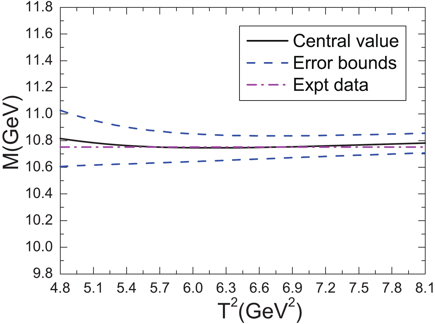
Figure 1. (color online) The mass of the vector hidden-bottom tetraquark candidate
$ Y(10750) $ as function of the Borel parameter$ T^2 .$ 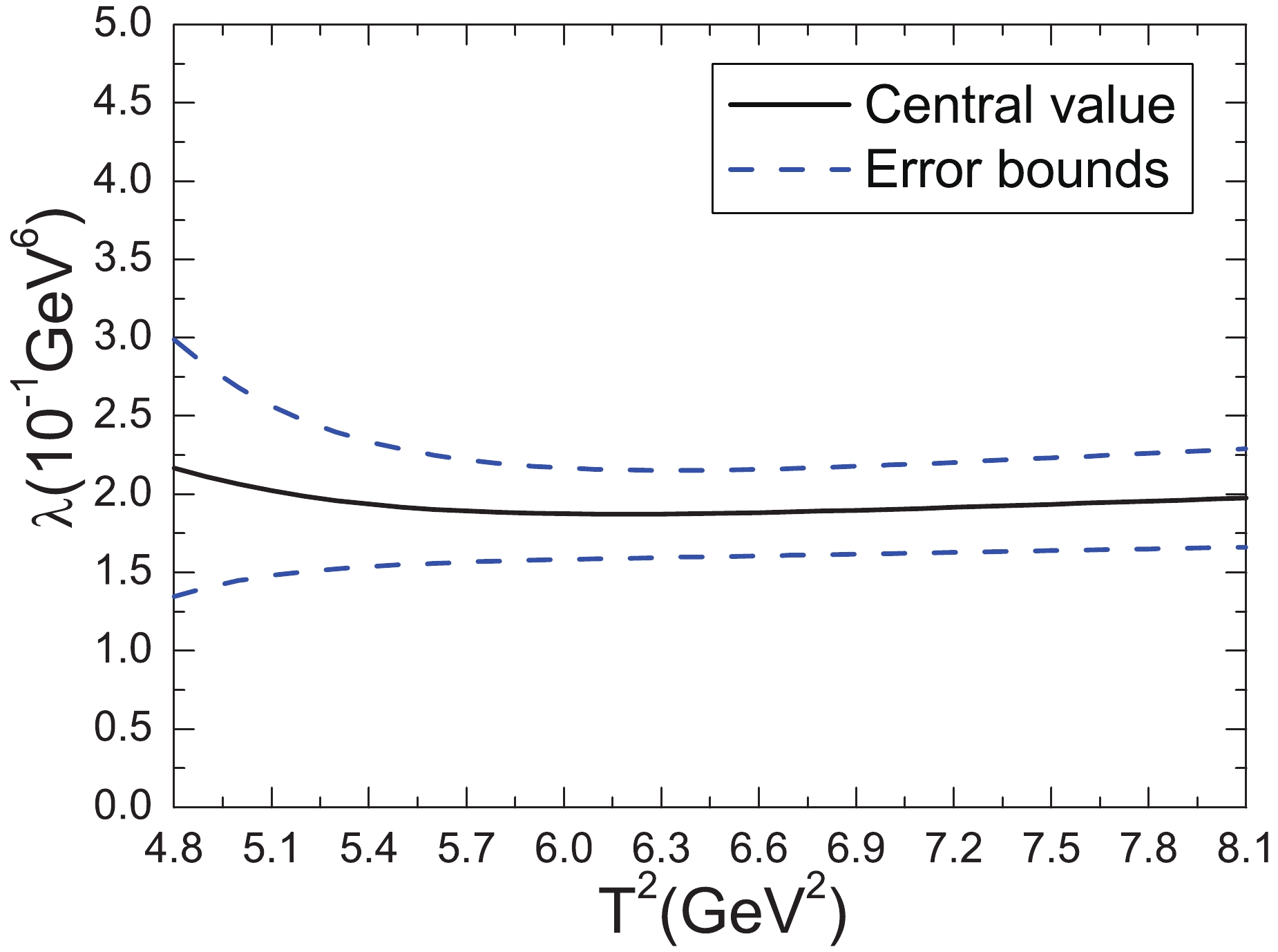
Figure 2. (color online) The pole residue of the vector hidden-bottom tetraquark candidate
$ Y(10750) $ as function of the Borel parameter$ T^2 .$ $ \begin{split} M_{Y} =& 10.75\pm0.10\,\rm{GeV} \, , \\ \lambda_{Y} = &\left( 1.89 \pm0.31 \right) \times 10^{-1}\,\rm{GeV}^6 \, . \end{split} $

(11) It is obvious from Figs.1-2 that both the mass and pole residue are on platforms in the Borel window. The four criteria of the QCD sum rules for the vector tetraquark states are all satisfied [15, 20, 21], and we expect to make reliable and reasonable predictions.
The numerical value
$ M_{Y} = 10.75\pm0.10\,\rm{GeV} $ from the QCD sum rules is in excellent agreement with (or at least compatible with) the experimental value of$M_Y = $ $ 10752.7\pm5.9\,{}^{+0.7}_{-1.1}\,\rm{MeV} $ obtained by the Belle collaboration [1] (see Fig. 1), which favors the assignment of$ Y(10750) $ as the diquark-antidiquark type vector hidden-bottom tetraquark state with a relative P-wave between the diquark and antidiquark constituents. The relative P-wave between the constituents hampers the rearrangement of quarks and antiquarks in the color and Dirac spinor spaces in order to form the quark-antiquark type meson pairs, which can explain (or is compatible with) the small experimental value of the width$ \Gamma_Y = 35.5^{+17.6}_{-11.3}\,{}^{+3.9}_{-3.3} $ MeV [1].In the charm sector, the calculations based on the QCD sum rules favor the assignments of
$ Y(4220/4260) $ ,$ Y(4320/4360) $ and$ Y(4390) $ as the vector tetraquark states with a relative P-wave between the scalar (or axial-vector) diquark and scalar (or axial-vector) antidiquark pair [6, 7]. Furthermore, the QCD sum rules favor the assignment of$ X^*(3860) $ as the scalar-diquark-scalar-antidiquark type scalar tetraquark state, where the diquark and antidiquark constituents are in the relative S-wave [25]. Analogous arguments also hold in the bottom and charm sectors, but unambiguous assignments require more experimental data and more theoretical work.In Fig. 3, we plot the predicted mass of the vector hidden-bottom tetraquark candidate
$ Y(10750) $ as function of the energy scale$ \mu $ for the central values of the input parameters. From the figure, we can see that the predicted mass decreases monotonically and quickly with increasing energy scale$ \mu $ . If we disregard the modified energy scale formula$ \mu = \sqrt{M^2_{X/Y/Z}-(2{\mathbb{M}}_Q+{P_E})^2} $ , it is not clear which energy scale should be chosen. If we choose the typical energy scale$ \mu = 2\,\rm{GeV} $ , which results in a pole contribution of 47%–70% and the$ D_{10} $ contribution of 2%–6%, we have to increase the continuum threshold parameter to a much larger value$ \sqrt{s_0} = 11.75\pm0.10\,\rm{GeV} $ to obtain the Borel window$ T^2 = (6.6-7.6)\,\rm{GeV}^2 $ , and the central values of the predicted mass and pole residue are$ M_Y = 11.20\,\rm{GeV} $ and$ \lambda_Y = 2.13\times 10^{-1}\,\rm{GeV}^{6} $ . The predicted mass$ M_Y = 11.20\,\rm{GeV} $ is much larger than the experimental value of$ M_Y = 10752.7\pm5.9\,{}^{+0.7}_{-1.1}\,\rm{MeV} $ obtained by the Belle collaboration [1]. The modified energy scale formula can enhance the pole contribution and improve the convergence behavior of the operator product expansion. On the other hand, if we choose the typical energy scale$ \mu = 3\,\rm{GeV} $ , the calculations lead to a mass of about$ 10.42\,\rm{GeV} $ , which is smaller than the S-wave hidden-bottom tetraquark masses$ 10.61-10.65\,\rm{GeV} $ [11], and hence should be rejected.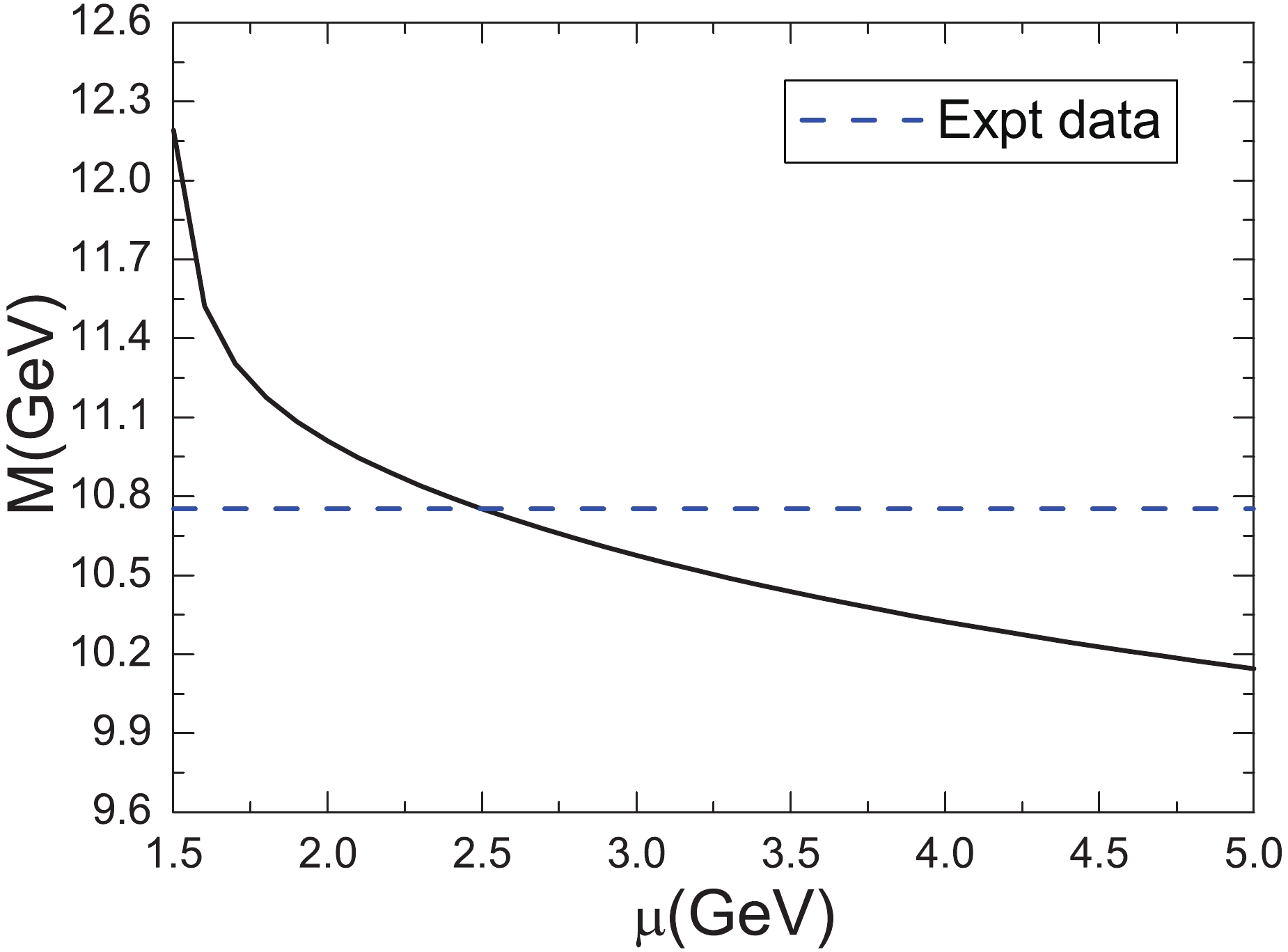
Figure 3. (color online) The predicted mass of the vector hidden-bottom tetraquark candidate
$ Y(10750) $ as function of the energy scale$ \mu $ for the central values of the input parameters. -
We now turn to the study of the partial decay widths of
$ Y(10750) $ as a vector hidden-bottom tetraquark candidate with the three-point QCD sum rules, and write down the three-point correlation functions,$ \begin{split} \Pi_{\nu}(p,q) =& i^2\int {\rm d}^4x{\rm d}^4y {\rm e}^{{\rm i}px}{\rm e}^{{\rm i}qy}\langle 0|T\Big\{J_{B}(x)J_{B}^{\dagger}(y)J_{\nu}^{\dagger}(0)\Big\}|0\rangle\, , \\ \Pi^1_{\alpha\beta\nu}(p,q) =& i^2\int {\rm d}^4x{\rm d}^4y {\rm e}^{{\rm i}px}{\rm e}^{{\rm i}qy}\langle 0|T\Big\{J_{B^*,\alpha}(x)J^{\dagger}_{B^*,\beta}(y)J_{\nu}^{\dagger}(0)\Big\}|0\rangle\, , \\ \Pi^1_{\mu\nu}(p,q) =& i^2\int {\rm d}^4x{\rm d}^4y {\rm e}^{{\rm i}px}{\rm e}^{{\rm i}qy}\langle 0|T\Big\{J_{B^*,\mu}(x)J_{B}^{\dagger}(y)J_{\nu}^{\dagger}(0)\Big\}|0\rangle\, , \\ \Pi^2_{\mu\nu}(p,q) =& i^2\int {\rm d}^4x{\rm d}^4y {\rm e}^{{\rm i}px}{\rm e}^{{\rm i}qy}\langle 0|T\Big\{J_{\eta_b}(x)J_{\omega,\mu}(y)J_{\nu}^{\dagger}(0)\Big\}|0\rangle\, ,\\ \Pi^3_{\mu\nu}(p,q) =& i^2\int {\rm d}^4x{\rm d}^4y {\rm e}^{{\rm i}px}{\rm e}^{{\rm i}qy}\langle 0|T\Big\{J_{\Upsilon,\mu}(x)J_{f_0}(y)J_{\nu}^{\dagger}(0)\Big\}|0\rangle\, ,\\ \Pi^2_{\alpha\beta\nu}(p,q) =& i^2\int {\rm d}^4x{\rm d}^4y {\rm e}^{{\rm i}px}{\rm e}^{{\rm i}qy}\langle 0|T\Big\{J_{\Upsilon,\alpha}(x)J_{\omega,\beta}(y)J_{\nu}^{\dagger}(0)\Big\}|0\rangle\, , \end{split} $

(12) where
$ \begin{split} J_{B}(x) = &\bar{b}(x)i\gamma_5 u(x) \, , \\ J_{B^*,\alpha}(x) = &\bar{b}(x)\gamma_\alpha u(x) \, , \\ J_{\eta_b}(x) = &\bar{b}(x)i\gamma_5 b(x)\, ,\\ J_{\omega,\mu}(y) =& \frac{\bar{u}(y)\gamma_\mu u(y)+\bar{d}(y)\gamma_\mu d(y)}{\sqrt{2}}\, , \\ J_{\Upsilon,\mu}(x) =& \bar{b}(x)\gamma_\mu b(x)\, ,\\ J_{f_0}(y) = &\frac{\bar{u}(y) u(y)+\bar{d}(y) d(y)}{\sqrt{2}}\, ,\\ J_\nu(0) =& J_\nu^{(0,0)}(0)\, . \end{split} $

(13) On the phenomenological side, we insert a complete set of intermediate hadronic states with the same quantum numbers as the current operators into the three-point correlation functions, and isolate the ground state contributions [12- 14],
$ \begin{split} \Pi_{\nu}(p,q) = & \frac{f_{B}^2m_{B}^4}{m_b^2}\frac{ \lambda_Y\,G_{YBB}}{\left(p^{\prime2}-m_Y^2\right)\left(p^2-m_{B}^2 \right)\left(q^2-m_{B}^2\right)}\\&\times i\,\left(p-q\right)^\alpha\left(-g_{\alpha\nu}+\frac{p^{\prime}_{\alpha}p^\prime_{\nu}}{p^{\prime2}}\right)+\cdots\\ =& \Pi(p^{\prime2},p^2,q^2)\,\left( -ip_{\nu}\right)+\cdots \, , \end{split} $

(14) $ \begin{split} \Pi^1_{\alpha\beta\nu}(p,q) = & \frac{f^2_{B^*}m^2_{B^*}\,\lambda_Y\,G_{YB^*B^*}}{\left(p^{\prime2}-m_Y^2\right)\left(p^2-m_{B^*}^2 \right)\left(q^2-m_{B^*}^2\right)}(-i)\left(p-q\right)^\sigma \\&\times \left(-g_{\nu\sigma}+\frac{p^{\prime}_{\nu}p^\prime_{\sigma}}{p^{\prime2}}\right) \left(-g_{\alpha\rho} +\frac{p_{\alpha}p_{\rho}}{p^2}\right)\\&\times \left(-g_{\beta}{}^\rho+\frac{q_{\beta}q^{\rho}}{q^2}\right)+\cdots\\ =& \Pi(p^{\prime2},p^2,q^2)\,\left( i g_{\alpha\beta}p_\nu\right)+\cdots \, , \end{split} $

(15) $ \begin{split} \Pi^1_{\mu\nu}(p,q) = & \frac{f_{B}m_{B}^2}{m_b}\frac{f_{B^*}m_{B^*}\,\lambda_Y\,G_{YBB^*}\,\varepsilon_{\alpha\beta\rho\sigma}p^\alpha p^{\prime\rho}}{\left(p^{\prime2}-m_Y^2\right)\left(p^2-m_{B^*}^2 \right)\left(q^2-m_{B}^2\right)}\,\\&\times i\,\left(-g_{\mu}{}^{\beta}+\frac{p_{\mu}p^{\beta}}{p^2}\right)\left(-g_{\nu}{}^{\sigma}+\frac{p^\prime_{\nu}p^{\prime\sigma}}{p^{\prime2}}\right)+\cdots\\ =& \Pi(p^{\prime2},p^2,q^2)\,\left(-i\varepsilon_{\mu\nu\alpha\beta}p^{\alpha}q^{\beta}\right)+\cdots \, , \end{split} $

(16) $ \begin{split} \Pi^2_{\mu\nu}(p,q) = & \frac{f_{\eta_b}m_{\eta_b}^2}{2m_b}\frac{f_{\omega}m_{\omega}\,\lambda_Y\,G_{Y\eta_b\omega}\,\varepsilon_{\alpha\beta\rho\sigma}q^\alpha p^{\prime\rho}}{\left(p^{\prime2}-m_Y^2\right)\left(p^2-m_{\eta_b}^2 \right)\left(q^2-m_{\omega}^2\right)}\\&\times (-i)\left(-g_{\mu}{}^{\beta}+\frac{q_{\mu}q^{\beta}}{q^2}\right)\left(-g_\nu{}^\sigma+\frac{p^\prime_{\nu}p^{\prime\sigma}}{p^{\prime2}}\right)+\cdots\\ =& \Pi(p^{\prime2},p^2,q^2)\left(-i\varepsilon_{\mu\nu\alpha\beta}p^{\alpha}q^{\beta}\right)+\cdots \, , \end{split} $

(17) $ \begin{split} \Pi^3_{\mu\nu}(p,q) = & \frac{f_{\Upsilon}m_{\Upsilon}f_{f_0}m_{f_0}\,\lambda_Y\,G_{Y\Upsilon f_0}}{\left(p^{\prime2}-m_Y^2\right)\left(p^2-m_{\Upsilon}^2 \right)\left(q^2-m_{f_0}^2\right)}\,\\&\times i\,\left(-g_{\mu\alpha}+\frac{p_{\mu}p_{\alpha}}{p^2}\right)\left(-g_\nu{}^\alpha+\frac{p^\prime_{\nu}p^{\prime\alpha}}{p^{\prime2}}\right)+\cdots\\ =& \Pi(p^{\prime2},p^2,q^2)\,\left(i g_{\mu\nu}\right) +\cdots \, , \end{split} $

(18) $ \begin{split} \Pi^2_{\alpha\beta\nu}(p,q) = & \frac{f_{\Upsilon}m_{\Upsilon}f_{\omega}m_{\omega}\,\lambda_Y\,G_{Y\Upsilon\omega}}{\left(p^{\prime2}-m_Y^2\right)\left(p^2-m_{\Upsilon}^2 \right)\left(q^2-m_{\omega}^2\right)}\\&\times(-i)\left(p-q\right)^\sigma \left(-g_{\nu\sigma}+\frac{p^{\prime}_{\nu}p^\prime_{\sigma}}{p^{\prime2}}\right) \left(-g_{\alpha\rho} +\frac{p_{\alpha}p_{\rho}}{p^2}\right)\\& \times \left(-g_{\beta}{}^\rho+\frac{q_{\beta}q^{\rho}}{q^2}\right)+\cdots\\ =& \Pi(p^{\prime2},p^2,q^2)\,\left( i g_{\alpha\beta}p_\nu\right)+\cdots \, , \end{split} $

(19) where we use the definitions for the decay constants and hadronic coupling constants,
$ \begin{split} \langle 0|J_{B}(0)|B(p)\rangle =& \frac{f_{B}m_{B}^2}{m_b}\, ,\\ \langle 0|J_{B^*,\mu}(0)|B^*(p)\rangle =& f_{B^*}m_{B^*}\xi^{B^*}_\mu\, ,\\ \langle 0|J_{\eta_b}(0)|\eta_b(p)\rangle =& \frac{f_{\eta_b}m_{\eta_b}^2}{2m_b}\, ,\\ \langle 0|J_{\Upsilon,\mu}(0)|\Upsilon(p)\rangle =& f_{\Upsilon}m_{\Upsilon}\xi^{\Upsilon}_\mu\, ,\\ \langle 0|J_{\omega,\mu}(0)|\omega(p)\rangle =& f_{\omega}m_{\omega}\xi^{\omega}_\mu\, ,\\ \langle 0|J_{f_0}(0)|f_0(p)\rangle =& f_{f_0}m_{f_0}\, , \end{split} $

(20) $ \begin{split} \langle B(p)B(q)|X(p^\prime)\rangle =& -(p-q)^\alpha\xi_\alpha^{Y}\, G_{YBB}\, ,\\ \langle B^*(p)B^*(q)|X(p^\prime)\rangle =& (p-q)^\alpha\xi_\alpha^{Y}\xi^{B^* *}_\beta\xi^{B^* *\beta}\, G_{YB^* B^*}\, ,\\ \langle B^*(p) B(q)|X(p^\prime)\rangle =& -\varepsilon^{\alpha\beta\rho\sigma}\,p_\alpha \xi^{B^* *}_{\beta}p^{\prime}_\rho\xi_\sigma^{Y}\, G_{YBB^* }\, , \\ \langle \eta_b(p)\omega(q)|X(p^\prime)\rangle =& \varepsilon^{\alpha\beta\rho\sigma}\,q_\alpha \xi^{\omega*}_{\beta}p^{\prime}_\rho\xi_\sigma^{Y}\, G_{Y\eta_b \omega}\, ,\\ \langle \Upsilon(p)f_0(q)|X(p^\prime)\rangle =& -\xi^{*\alpha}_{\Upsilon}\xi_\alpha^{Y}\, G_{Y\Upsilon f_0}\, ,\\ \langle \Upsilon(p)\omega(q)|X(p^\prime)\rangle =& (p-q)^\alpha\xi_\alpha^{Y}\xi^{\Upsilon *}_\beta\xi^{\omega *\beta}\, G_{Y\Upsilon \omega}\, , \end{split} $

(21) $ \xi^{B^*}_\mu $ ,$ \xi^{\Upsilon}_\mu $ ,$ \xi^{\omega}_\mu $ and$ \xi^{Y}_\mu $ are the polarization vectors of the conventional mesons and the tetraquark candidate$ Y(10750) $ , respectively, and$ G_{YBB} $ ,$ G_{YB^*B^*} $ ,$ G_{YBB^*} $ ,$ G_{Y\eta_b \omega} $ ,$ G_{Y\Upsilon f_0} $ and$ G_{Y\Upsilon\omega} $ are the hadronic coupling constants. In the calculations, we observed that the hadronic coupling constant$ G_{Y\Upsilon\omega} $ is zero at the leading order approximation, and so we neglect the process$ Y(10750)\to \Upsilon\,\omega\to \Upsilon\pi^+\pi^-\pi^0 $ .The lowest scalar nonet mesons
$ \{f_0/\sigma(500),a_0(980), $ $\kappa_0(800),f_0(980) \} $ are usually assigned as the tetraquark states, and the higher scalar nonet mesons$ \{f_0(1370),a_0(1450),K^*_0(1430),f_0(1500) \} $ as the conventional$ {}^3P_0 $ quark-antiquark states [26-28]. Here, we assume$ f_0 = f_0(1370) $ with the symbolic quark structure$ f_0(1370) = \dfrac{\bar{u}u+\bar{d}d}{\sqrt{2}} $ .Considering the components
$ \Pi(p^{\prime2},p^2,q^2) $ of the correlation functions in Eqs. (14)-(19), we carry out the operator product expansion up to the vacuum condensates of dimension 5. We then calculate the connected and disconnected Feynman diagrams taking into account the perturbative terms, quark condensate and mixed condensate, and neglect the tiny contributions of the gluon condensate. We obtain the QCD spectral densities from the dispersion relation, where we match the hadron side with the QCD side of the components$ \Pi(p^{\prime2},p^2,q^2) $ , and perform the double Borel transform with respect to$ P^2 = -p^2 $ and$ Q^2 = -q^2 $ setting$ p^{\prime2} = p^2 $ in the hidden-bottom channels and$ p^{\prime2} = 4p^2 $ in the open-bottom channels. The QCD sum rules for the hadronic coupling constants are then,$ \begin{split}& \frac{f_{B}^2m_{B}^4}{m_b^2}\frac{ \lambda_Y\,G_{YBB}}{4\left(\widetilde{m}_Y^2-m_{B}^2\right)}\left[\exp\left(-\frac{m_{B}^2}{T_1^2}\right) -\exp\left(-\frac{\widetilde{m}_Y^2}{T_1^2}\right) \right]\exp\left( -\frac{m_{B}^2}{T_2^2}\right) +\left(C_{Y^{\prime}B^+}+C_{Y^{\prime}B^-} \right)\exp\left(-\frac{m_{B}^2}{T_1^2} -\frac{m_{B}^2}{T_2^2}\right)\\ =& -\frac{1}{512\pi^4}\int_{m_b^2}^{s^0_{B}} {\rm d}s \int_{m_b^2}^{s^0_{B}} {\rm d}u \left(1-\frac{m_b^2}{s}\right)^2\left(1-\frac{m_b^2}{u}\right)^2\frac{m_b^2}{s} \left(3s^2-5su-14s m_b^2+4u m_b^2\right) \exp\left(-\frac{s}{T_1^2}-\frac{u}{T_2^2}\right) \end{split} $ 
$ \begin{split}& -\frac{m_b\langle\bar{q}q\rangle}{192\pi^2} \int_{m_b^2}^{s^0_{B}} {\rm d}u\left(1-\frac{m_b^2}{u}\right)^2 \left(u+11m_b^2\right) \exp\left(-\frac{m_b^2}{T_1^2}-\frac{u}{T_2^2}\right) +\frac{m_b\langle\bar{q}q\rangle}{192\pi^2}\int_{m_b^2}^{s^0_{B}} {\rm d}s\left(1-\frac{m_b^2}{s}\right)^2 \left(3s-19m_b^2+\frac{4m_b^4}{s}\right) \exp\left(-\frac{s}{T_1^2}-\frac{m_b^2}{T_2^2}\right) \\ & -\frac{m_b\langle\bar{q}g_{s}\sigma Gq\rangle}{768\pi^2}\int_{m_b^2}^{s^0_{B}} {\rm d}u\left(1-\frac{m_b^2}{u}\right)^2 \left(27-\frac{u+29m_b^2}{T_1^2}\right) \exp\left(-\frac{m_b^2}{T_1^2}-\frac{u}{T_2^2}\right) -\frac{m_b^3\langle\bar{q}g_{s}\sigma Gq\rangle}{384\pi^2T_1^2}\int_{m_b^2}^{s^0_{B}} {\rm d}u\left(1-\frac{m_b^2}{u}\right)^2\\&\times \left(9-\frac{u+11m_b^2}{2T_1^2}\right) \exp\left(-\frac{m_b^2}{T_1^2}-\frac{u}{T_2^2}\right) -\frac{m_b\langle\bar{q}g_{s}\sigma Gq\rangle}{768\pi^2}\int_{m_b^2}^{s^0_{B}} {\rm d}s\left(1-\frac{m_b^2}{s}\right)^2 \left(1-\frac{4m_b^2}{s}\right) \left(1+\frac{3s-m_b^2}{T_2^2}\right)\exp\left(-\frac{s}{T_1^2}-\frac{m_b^2}{T_2^2}\right) \\ & -\frac{m_b^3\langle\bar{q}g_{s}\sigma Gq\rangle}{384\pi^2T_2^2}\int_{m_b^2}^{s^0_{B}} {\rm d}s\left(1-\frac{m_b^2}{s}\right)^2\left\{1-\frac{4m_b^2}{s} -\frac{1}{2T_2^2}\left[18m_b^2-3s+m_b^2\left(1-\frac{4m_b^2}{s}\right)\right]\right\} \exp\left(-\frac{s}{T_1^2}-\frac{m_b^2}{T_2^2}\right) \\ & -\frac{m_b\langle\bar{q}g_{s}\sigma Gq\rangle}{768\pi^2}\int_{m_b^2}^{s^0_{B}} {\rm d}u\left(1-\frac{m_b^2}{u}\right)^2 \left(-9+\frac{7u+11m_b^2}{T_1^2}\right) \exp\left(-\frac{m_b^2}{T_1^2}-\frac{u}{T_2^2}\right) \\ & -\frac{m_b\langle\bar{q}g_{s}\sigma Gq\rangle}{768\pi^2}\int_{m_b^2}^{s^0_{B}} {\rm d}s\left(1-\frac{m_b^2}{s}\right)^2 \left\{\frac{4m_b^2}{s}-1+\frac{1}{T_2^2}\left[24m_b^2-3s+\left(1-\frac{4m_b^2}{s}\right) m_b^2 \right]\right\} \exp\left(-\frac{s}{T_1^2}-\frac{m_b^2}{T_2^2}\right) \\ & +\frac{m_b\langle\bar{q}g_{s}\sigma Gq\rangle}{256\pi^2}\int_{m_b^2}^{s^0_{B}} {\rm d}u\left(1-\frac{m_b^2}{u}\right) \left(5-\frac{4m_b^2}{u}\right) \exp\left(-\frac{m_b^2}{T_1^2}-\frac{u}{T_2^2}\right) +\frac{m_b\langle\bar{q}g_{s}\sigma Gq\rangle}{128\pi^2}\int_{m_b^2}^{s^0_{B}} {\rm d}s\left(1-\frac{m_b^2}{s}\right) \left(2-\frac{5m_b^2}{s}+\frac{2m_b^4}{s^2}\right) \exp\left(-\frac{s}{T_1^2}-\frac{m_b^2}{T_2^2}\right) \\& -\frac{m_b\langle\bar{q}g_{s}\sigma Gq\rangle}{256\pi^2}\int_{m_b^2}^{s^0_{B}} {\rm d}s\left(1-\frac{3m_b^2}{s}+\frac{8m_b^4}{s^2}-\frac{2m_b^6}{s^3}\right) \exp\left(-\frac{s}{T_1^2}-\frac{m_b^2}{T_2^2}\right) \, , \end{split} $

(22) $ \begin{split}& \frac{f_{B^*}^2 m_{B^*}^2 \lambda_Y G_{YB^* B^*}}{4\left(\widetilde{m}_Y^2-m_{B^*}^2\right)} \left[\exp\left(-\frac{m_{B^*}^2}{T_1^2}\right)-\exp\left(-\frac{\widetilde{m}_Y^2}{T_1^2}\right)\right] \exp\left(-\frac{m_{B^*}^2}{T_2^2}\right) +C_{Y^{\prime}B^{*+}+Y^{\prime}B^{*-}}\exp\left(-\frac{m_{B^*}^2}{T_1^2}\right)\exp\left(-\frac{m_{B^*}^2}{T_2^2}\right) \\ =& \frac{1}{1536\pi^4}\int_{m_b^2}^{s^0_{B^*}} {\rm d}s \int_{m_b^2}^{s^0_{B^*}} {\rm d}u \left(1-\frac{m_b^2}{s}\right)^2 \left(1-\frac{m_b^2}{u}\right)^2 \frac{m_b^2}{s} \left(2m_b^4+46s m_b^2-8u m_b^2-9s^2+5su\right) \exp\left(-\frac{s}{T_1^2}-\frac{u}{T_2^2}\right) \\ & +\frac{m_b\langle\bar{q}q\rangle}{192\pi^2}\int_{m_b^2}^{s^0_{B^*}} {\rm d}u\left(1-\frac{m_b^2}{u}\right)^2 \left(u-13m_b^2\right) \exp\left(-\frac{m_b^2}{T_1^2}-\frac{u}{T_2^2}\right) +\frac{m_b\langle\bar{q}q\rangle}{192\pi^2}\int_{m_b^2}^{s^0_{B^*}} {\rm d}s\left(1-\frac{m_b^2}{s}\right)^2 \left(3s-17m_b^2+\frac{2m_b^4}{s}\right) \exp\left(-\frac{s}{T_1^2}-\frac{m_b^2}{T_2^2}\right) \\& -\frac{m_b\langle\bar{q}g_{s}\sigma Gq\rangle}{1152\pi^2}\int_{m_b^2}^{s^0_{B^*}} {\rm d}u\left(1-\frac{m_b^2}{u}\right)^2 \left(45+\frac{7u-55m_b^2}{T_1^2}\right)\exp\left(-\frac{m_b^2}{T_1^2}-\frac{u}{T_2^2}\right) +\frac{m_b^3\langle\bar{q}g_{s}\sigma Gq\rangle}{384\pi^2T_1^2}\int_{m_b^2}^{s^0_{B^*}} {\rm d}u \left(1-\frac{m_b^2}{u}\right)^2 \\& \times \left(-9+\frac{-u+13m_b^2}{2T_1^2}\right)\exp\left(-\frac{m_b^2}{T_1^2}-\frac{u}{T_2^2}\right) -\frac{m_b\langle\bar{q}g_{s}\sigma Gq\rangle}{576\pi^2}\int_{m_b^2}^{s^0_{B^*}} {\rm d}s \left(1-\frac{m_b^2}{s}\right)^2\left(1-\frac{4m_b^2}{s}\right)\left(1+\frac{3s-m_b^2}{T_2^2}\right) \exp\left(-\frac{s}{T_1^2}-\frac{m_b^2}{T_2^2}\right) \\& -\frac{m_b^3\langle\bar{q}g_{s}\sigma Gq\rangle}{384\pi^2T_2^2}\int_{m_b^2}^{s^0_{B^*}} {\rm d}s \left(1-\frac{m_b^2}{s}\right)^2\left(1-\frac{4m_b^2}{s}\right)\exp\left(-\frac{s}{T_1^2}-\frac{m_b^2}{T_2^2}\right) \\& +\frac{m_b^3\langle\bar{q}g_{s}\sigma Gq\rangle}{768\pi^2T_2^4}\int_{m_b^2}^{s^0_{B^*}} {\rm d}s \left(1-\frac{m_b^2}{s}\right)^2\left[-3s+16m_b^2+\frac{2m_b^4}{s}+\left(1-\frac{4m_b^2}{s}\right)m_b^2\right] \exp\left(-\frac{s}{T_1^2}-\frac{m_b^2}{T_2^2}\right) \\& +\frac{m_b\langle\bar{q}g_{s}\sigma Gq\rangle}{768\pi^2}\int_{m_b^2}^{s^0_{B^*}} {\rm d}s\left(1-\frac{m_b^2}{s}\right)\left(13-\frac{35m_b^2}{s}+\frac{16m_b^4}{s^2}\right) \exp\left(-\frac{s}{T_1^2}-\frac{m_b^2}{T_2^2}\right) \\ &+\frac{m_b\langle\bar{q}g_{s}\sigma Gq\rangle}{768\pi^2}\int_{m_b^2}^{s^0_{B^*}} {\rm d}u\left(1-\frac{m_b^2}{u}\right) \left(5-\frac{32m_b^2}{u}\right)\exp\left(-\frac{m_b^2}{T_1^2}-\frac{u}{T_2^2}\right) \\ &+\frac{m_b\langle\bar{q}g_{s}\sigma Gq\rangle}{2304\pi^2}\int_{m_b^2}^{s^0_{B^*}} {\rm d}s \left(4-\frac{9m_b^2}{s}+\frac{27m_b^4}{s^2}-\frac{10m_b^6}{s^3}\right)\exp\left(-\frac{s}{T_1^2}-\frac{m_b^2}{T_2^2}\right)\, , \end{split} $

(23) $ \begin{split} & \frac{f_{B^*}f_B m_{B^*}m_B^2 \lambda_Y G_{YB^* B}}{4m_b \left(\widetilde{m}_Y^2-m_{B^*}^2\right)} \left[\exp\left(-\frac{m_{B^*}^2}{T_1^2}\right)-\exp\left(-\frac{\widetilde{m}_Y^2}{T_1^2}\right)\right] \exp\left(-\frac{m_B^2}{T_2^2}\right) +C_{Y^{\prime}B^{*+}+Y^{\prime}B^-}\exp\left(-\frac{m_{B^*}^2}{T_1^2}\right)\exp\left(-\frac{m_B^2}{T_2^2}\right) \\ =& \frac{m_b}{256\pi^4}\int_{m_b^2}^{s^0_{B^*}} {\rm d}s \int_{m_b^2}^{s^0_{B}} {\rm d}u \left(1-\frac{m_b^2}{s}\right)^2\left(1-\frac{m_b^2}{u}\right)^2\left(s+u-2m_b^2\right) \exp\left(-\frac{s}{T_1^2}-\frac{u}{T_2^2}\right) \\ & -\frac{\langle\bar{q}q\rangle}{96\pi^2}\int_{m_b^2}^{s^0_{B}} {\rm d}u\left(1-\frac{m_b^2}{u}\right)^2 \left(u-m_b^2\right) \exp\left(-\frac{m_b^2}{T_1^2}-\frac{u}{T_2^2}\right) -\frac{\langle\bar{q}q\rangle}{96\pi^2}\int_{m_b^2}^{s^0_{B^*}} {\rm d}s\left(1-\frac{m_b^2}{s}\right)^2 \left(s-m_b^2\right) \exp\left(-\frac{s}{T_1^2}-\frac{m_b^2}{T_2^2}\right) \\ & +\frac{\langle\bar{q}g_{s}\sigma Gq\rangle}{288\pi^2T_1^2}\left(1+\frac{3m_b^2}{4T^2_1}\right)\int_{m_b^2}^{s^0_{B}} {\rm d}u\left(1-\frac{m_b^2}{u}\right)^2 \left(u-m_b^2\right)\exp\left(-\frac{m_b^2}{T_1^2}-\frac{u}{T_2^2}\right) +\frac{m_b^2\langle\bar{q}g_{s}\sigma Gq\rangle}{384\pi^2T_2^4}\int_{m_b^2}^{s^0_{B^*}} {\rm d}s \left(1-\frac{m_b^2}{s}\right)^2\\ &\times \left(s-m_b^2\right)\exp\left(-\frac{s}{T_1^2}-\frac{m_b^2}{T_2^2}\right) +\frac{\langle\bar{q}g_{s}\sigma Gq\rangle}{384\pi^2}\int_{m_b^2}^{s^0_{B}} {\rm d}u \left(1-\frac{m_b^2}{u}\right)\left(-1+\frac{2m_b^2}{u}\right)\exp\left(-\frac{m_b^2}{T_1^2}-\frac{u}{T_2^2}\right) \\& +\frac{\langle\bar{q}g_{s}\sigma Gq\rangle}{384\pi^2}\int_{m_b^2}^{s^0_{B^*}} {\rm d}s \left(1-\frac{m_b^2}{s}\right)\left(2-\frac{m_b^2}{s}\right) \exp\left(-\frac{s}{T_1^2}-\frac{m_b^2}{T_2^2}\right) \, , \end{split} $

(24) $ \begin{split}& \frac{f_{\eta_b}f_{\omega} m_{\eta_b}^2 m_{\omega} \lambda_Y G_{Y\eta_b \omega}}{2m_b \left(m_Y^2-m_{\eta_b}^2\right)} \left[\exp\left(-\frac{m_{\eta_b}^2}{T_1^2}\right)-\exp\left(-\frac{m_Y^2}{T_1^2}\right)\right] \exp\left(-\frac{m_{\omega}^2}{T_2^2}\right) +C_{Y^{\prime}\eta_b+Y^{\prime}\omega}\exp\left(-\frac{m_{\eta_b}^2}{T_1^2}\right)\exp\left(-\frac{m_{\omega}^2}{T_2^2}\right) \\ =& \frac{m_b}{64\sqrt{2}\pi^4}\int_{4m_b^2}^{s^0_{\eta_b}} {\rm d}s \int_{0}^{s^0_{\omega}} {\rm d}u \sqrt{1-\frac{4m_b^2}{s}}\, u\, \exp\left(-\frac{s}{T_1^2}-\frac{u}{T_2^2}\right) -\frac{\langle\bar{q}q\rangle}{24\sqrt{2}\pi^2}\int_{4m_b^2}^{s^0_{\eta_b}} {\rm d}s\sqrt{1-\frac{4m_b^2}{s}}\left(s-4m_b^2\right) \exp\left(-\frac{s}{T_1^2}\right) \\ &+\frac{\langle\bar{q}g_{s}\sigma Gq\rangle}{72\sqrt{2}\pi^2T_2^2}\int_{4m_b^2}^{s^0_{\eta_b}} {\rm d}s \sqrt{1-\frac{4m_b^2}{s}}\left(s-4m_b^2\right)\exp\left(-\frac{s}{T_1^2}\right) -\frac{\langle\bar{q}g_{s}\sigma Gq\rangle}{96\sqrt{2}\pi^2}\int_{4m_b^2}^{s^0_{\eta_b}} {\rm d}s \sqrt{1-\frac{4m_b^2}{s}}\exp\left(-\frac{s}{T_1^2}\right) \, , \end{split} $

(25) $ \begin{split}& \frac{f_{\Upsilon}f_{f} m_{\Upsilon} m_{f} \lambda_Y G_{Y\Upsilon f_0}}{m_Y^2-m_{\Upsilon}^2} \left[\exp\left(-\frac{m_{\Upsilon}^2}{T_1^2}\right)-\exp\left(-\frac{m_Y^2}{T_1^2}\right)\right] \exp\left(-\frac{m_{f_0}^2}{T_2^2}\right) +C_{Y^{\prime}\Upsilon+Y^{\prime}f_0}\exp\left(-\frac{m_{\Upsilon}^2}{T_1^2}\right)\exp\left(-\frac{m_{f_0}^2}{T_2^2}\right) \\ =& \frac{m_b}{128\sqrt{2}\pi^4}\int_{4m_b^2}^{s^0_{\Upsilon}} {\rm d}s \int_{0}^{s^0_{f_0}} {\rm d}u \sqrt{1-\frac{4m_b^2}{s}}\, u\, \left(u+2s-8m_b^2\right)\exp\left(-\frac{s}{T_1^2}-\frac{u}{T_2^2}\right) \\ &+\frac{\langle\bar{q}g_{s}\sigma Gq\rangle}{48\sqrt{2}\pi^2}\int_{4m_b^2}^{s^0_{\Upsilon}} {\rm d}s\sqrt{1-\frac{4m_b^2}{s}} \left(s+2m_b^2\right)\exp\left(-\frac{s}{T_1^2}\right)\, , \end{split} $

(26) where
$ \widetilde{m}_Y^2 = \dfrac{m_Y^2}{4} $ , the unknown functions$ C_{Y^{\prime}B^+}+C_{Y^{\prime}B^-} $ ,$ C_{Y^{\prime}B^{*+}+Y^{\prime}B^{*-}} $ ,$ C_{Y^{\prime}B^{*+}+Y^{\prime}B^-} $ ,$ C_{Y^{\prime}\eta_b+Y^{\prime}\omega} $ and$ C_{Y^{\prime}\Upsilon+Y^{\prime}f_0} $ parametrize the transitions between the ground states (B,$ B^* $ ,$ \Upsilon $ ,$ \eta_b $ ,$ \omega $ ,$ f_0(1370) $ ) and the excited states$ Y^\prime $ . The definitions of the unknown functions and the technical details of the calculations can be found in Refs. [29-32].The input parameters for the hadron side are chosen as
$ m_{\Upsilon} = 9.4603\,\rm{GeV} $ ,$ m_{\eta_b} = 9.3987\,\rm{GeV} $ ,$ m_{\omega} = 0.78265\,\rm{GeV} $ ,$ m_{B^+} = 5.27925\,\rm{GeV} $ ,$ m_{B^{*+}} = 5.3247\,\rm{GeV} $ ,$ m_{\pi^+} = 0.13957\,\rm{GeV} $ ,$ \sqrt{s^0_{B}} = 5.8\,\rm{GeV} $ ,$ \sqrt{s^0_{B^*}} = 5.8\,\rm{GeV} $ ,$ \sqrt{s^0_{\Upsilon}} = 9.9\,\rm{GeV} $ ,$ \sqrt{s^0_{\eta_b}} = 9.9\,\rm{GeV} $ [17],$ \sqrt{s^0_{\omega}} = 1.3\,\rm{GeV} $ ,$ f_{\omega} = 215\,\rm{MeV} $ [33],$ m_{f_0} = 1.35\,\rm{GeV} $ ,$ f_{f_0} = 546\,\rm{MeV} $ ,$ \sqrt{s^0_{f_0}} = 1.8\,\rm{GeV} $ (This work),$ f_{B} = 194\,\rm{MeV} $ ,$ f_{B^*} = 213\,\rm{MeV} $ [34, 35],$ f_{\Upsilon} = 649\,\rm{MeV} $ [36],$ f_{\eta_b} = 667\,\rm{MeV} $ [37].We set the Borel parameters to
$ T_1^2 = T_2^2 = T^2 $ for simplicity of the QCD sum rules for the hadronic coupling constants$ G_{YBB} $ ,$ G_{YB^*B^*} $ ,$ G_{YB^*B} $ and$ G_{Y\eta_b\omega} $ . In the QCD sum rules for the hadronic coupling constant$ G_{Y\Upsilon f_0} $ , the contribution of the u channel can be factorized out explicitly, and we take the local limit, i.e.$ T_2^2 \to \infty $ and$ T_1^2 = T^2 $ . The unknown parameters are chosen as$ \begin{aligned} C_{Y^{\prime}B^+}+C_{Y^{\prime}B^-}& = 0.0441\;{\rm{GeV}}^8,\;C_{Y^{\prime}B^{*+}+Y^{\prime}B^{*-}} = 0.0454\;{\rm{GeV}}^8\\ C_{Y^{\prime}B^{*+}+Y^{\prime}B^-} & = 0.00145 \:{\rm{GeV}}^7,\;C_{Y^{\prime}\eta_b+Y^{\prime}\omega} = 0.0000125\;{\rm{GeV}}^7\\ {\rm{and}}\; C_{Y^{\prime}\Upsilon+Y^{\prime}f_0} &= 0.00238\;{\rm{GeV}}^9 \end{aligned}$

to obtain platforms in the Borel windows, shown in Table 1. In Fig. 4, we plot the hadronic coupling constants G as function of the Borel parameter
$ T^2 $ in the Borel windows. The Borel windows are$ T_{\max}^2-T^2_{\min} = 1.0\,\rm{GeV}^2 $ for the hidden-bottom decays, and$ T_{\max}^2-T^2_{\min} = 0.8\,\rm{GeV}^2 $ for the open-bottom decays, where$ T^2_{\max} $ and$ T^2_{\min} $ denote the maximum and minimum of the Borel parameter. We choose the same intervals$ T_{\max}^2-T^2_{\min} $ in all QCD sum rules for the hadronic coupling constants in the two-body strong decays [29-32], which works well for the decays of$ Z_c(3900) $ ,$ X(4140) $ ,$ Z_c(4600) $ ,$ Y(4660) $ , etc.$ T^2/\rm{GeV}^2 $ 

G $ \Gamma/\rm{MeV} $ 

$ Y(10750)\to B^+B^- $ 

$ 5.1-5.9 $ 

$ 3.70^{+1.51}_{-1.31} $ 

$ 6.61^{+6.50}_{-3.85} $ 

$ Y(10750)\to B^{*+}B^{*-} $ 

$ 5.5-6.3 $ 

$ 3.89^{+1.68}_{-1.45} $ 

$ 8.79^{+9.23}_{-5.33} $ 

$ Y(10750)\to B^{*+}B^{-} $ 

$ 4.0-4.8 $ 

$ \sim0.01\,\rm{GeV}^{-1} $ 

$ \sim 0.02 $ 

$ Y(10750)\to \eta_b\, \omega $ 

$ 2.6-3.6 $ 

$ 0.30^{+0.20}_{-0.12}\,\rm{GeV}^{-1} $ 

$ 2.64^{+4.70}_{-1.69} $ 

$ Y(10750)\to \Upsilon f_0(1370)\to \Upsilon \pi^+\pi^- $ 

$ 2.5-3.5 $ 

$ 1.32^{+1.10}_{-0.60}\,\rm{GeV} $ 

$ 0.08^{+0.20}_{-0.06} $ 

$ Y(10750)\to \Upsilon \omega $ 

$ \sim 0 $ 

$ \sim 0 $ 

Table 1. The Borel windows, hadronic coupling constants and partial decay widths of
$ Y(10750) $ as the vector hidden-bottom tetraquark state.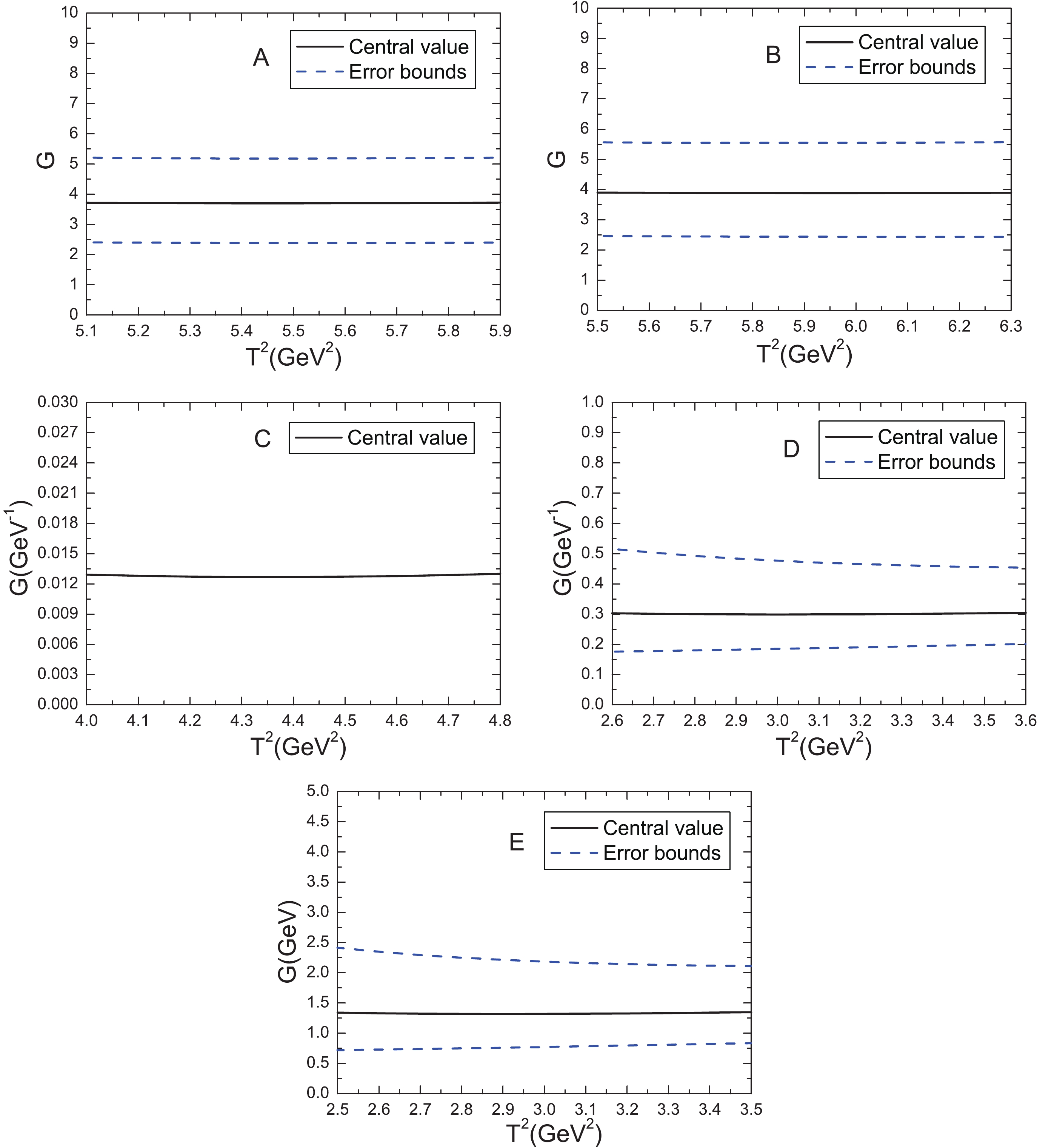
Figure 4. (color online) The hadronic coupling constants as function of the Borel parameter
$ T^2 $ . A, B, C, D and E denote the hadronic coupling constants$ G_{YBB} $ ,$ G_{YB^*B^*} $ ,$ G_{YB^*B} $ ,$ G_{Y\eta_b\omega} $ and$ G_{Y\Upsilon f_0} $ , respectively.We take into account the uncertainties of the input parameters, and obtain the hadronic coupling constants, as shown in Table 1 and Fig. 4. Due to the tiny value of the hadronic coupling constant
$ G_{YBB^*} $ , we neglect its uncertainty. The partial decay widths of the two-body strong decays$ Y(10750)\to B^+B^- $ ,$ B^{*+}B^{*-} $ ,$ B^{*+}B^- $ and$ \eta_b\omega $ are calculated with the formula,$ \begin{aligned} \Gamma\left(Y(10750)\to BC\right) = \frac{p(m_Y,m_B,m_C)}{24\pi m_Y^2} |T^2|\, , \end{aligned} $

(27) where
$ p(a,b,c) = \dfrac{\sqrt{[a^2-(b+c)^2][a^2-(b-c)^2]}}{2a} $ , and T is the scattering amplitude defined in Eq. (21). The numerical values of the partial decay widths are shown in Table 1.We assume that the three-body decay
$ Y(10750)\to $ $ \Upsilon f_0(1370)\to \Upsilon \pi^+\pi^- $ takes place through an intermediate virtual state$ f_0(1370) $ , and calculate the partial decay width,$ \begin{split} \Gamma(Y\to \Upsilon\pi^+\pi^-) =& \int_{4m_\pi^2}^{(m_Y-m_{\Upsilon})^2}{\rm d}s\,|T|^2\\&\times \frac{p(m_Y,m_{\Upsilon},\sqrt{s})\,p(\sqrt{s},m_\pi,m_\pi)}{192\pi^3 m_Y^2 \sqrt{s} }\, \\ =& 0.08^{+0.20}_{-0.06}\,\rm{MeV}\, , \end{split} $

(28) where
$ \begin{split} |T|^2 =& \frac{(M_Y^2-s)^2+2(5M_Y^2-s)M^2_{\Upsilon}+M^4_{\Upsilon}}{4M_Y^2 M_{\Upsilon}^2}\\&\times G_{Y\Upsilon f_0}^2\frac{1}{(s-m_{f_0}^2)^2+s\Gamma_{f_0}^2(s)}G_{f_0\pi\pi}^2\, , \\ \Gamma_{f_0}(s) =& \Gamma_{f_0}(m_{f_0}^2) \frac{m_{f_0}^2}{s}\sqrt{\frac{s-4m_{\pi}^2}{m_{f_0}^2-4m_{\pi}^2}}\, , \\ \Gamma_{f_0}(m_{f_0}^2) = & \frac{G_{f_0\pi\pi}^2}{16\pi m_{f_0}^2}\sqrt{ m_{f_0}^2-4m_{\pi}^2 }\, , \end{split} $

(29) $ \Gamma_{f_0}(m_{f_0}^2) = 200\,\rm{MeV} $ [17]. The hadronic coupling constant$ G_{f_0\pi\pi} $ is defined by$ \langle \pi^+(p)\pi^-(q)|f_0(p^\prime)\rangle = iG_{f_0\pi\pi} $ . If we take the largest width$ \Gamma_{f_0}(m_{f_0}^2) = 500\,\rm{MeV} $ [17], we can obtain a slightly larger partial decay width$ \Gamma(Y\to \Upsilon\pi^+\pi^-) = $ $ 0.11^{+0.27}_{-0.08}\,\rm{MeV} $ .It is now easy to obtain the total decay width,
$ \begin{split} \Gamma_{Y} = & \Gamma\left(Y(10750)\to B^+B^-,\,B^0\bar{B}^0, \, B^{*+}B^{*-}, \, B^{*0}\bar{B}^{*0}, \right.\\ & B^{*+}B^{-}, \, B^{+}B^{*-}, \left.B^{*0}\bar{B}^{0}, \, B^{0}\bar{B}^{*0},\, \eta_b\omega, \, \Upsilon\pi^+\pi^-\right)\, ,\\ =& 33.60^{+16.64}_{-9.45}\,{\rm{MeV}}\, , \end{split} $

(30) where we assume the isospin limit for the B and
$ B^* $ mesons. The predicted width$ \Gamma_{Y} = 33.60^{+16.64}_{-9.45}\,{\rm{MeV}} $ is in excellent agreement with the experimental value of$ 35.5^{+17.6}_{-11.3}\,{}^{+3.9}_{-3.3}\,\rm{MeV} $ obtained by the Belle collaboration [1], which also supports the assignment of$ Y(10750) $ as the diquark-antidiquark type vector hidden-bottom tetraquark state.In Ref. [5], Li et al. assigned
$ Y(10750) $ and$ \Upsilon(10860) $ as the$ 5^3{S}_1-4^3{D}_1 $ mixed state, where the dominant components of$ Y(10750) $ and$ \Upsilon(10860) $ are the conventional bottomonium sates$ 4^3{D}_1 $ and$ 5^3{S}_1 $ , respectively. The decay mode$ 4^3{D}_1 \to B^*B^* $ is the dominant mode, the decay mode$ 4^3{D}_1 \to BB^* $ is sizable, while the decay mode$ 4^3{D}_1 \to BB $ is nearly forbidden. In the present work, we assign$ Y(10750) $ as the vector hidden-bottom tetraquark state with dominant decay modes$ Y(10750)\to BB $ and$ B^*B^* $ , while the partial decay widths for the decay$ Y(10750) \to BB^* $ are tiny.$ Y(10750) $ could be searched for in the processes$ Y(10750)\to B^+B^- $ ,$ B^0\bar{B}^0 $ ,$ B^{*+}B^{*-} $ ,$ B^{*0}\bar{B}^{*0} $ ,$ B^{*+}B^{-} $ ,$ B^{+}B^{*-} $ ,$ B^{*0}\bar{B}^{0} $ ,$ B^{0}\bar{B}^{*0} $ ,$ \eta_b\omega $ ,$ \Upsilon\pi^+\pi^- $ to reveal its nature. -
In this article, we have taken the scalar diquark and scalar antidiquark operators as the basic constituents, and constructed the
$ C\gamma_5\otimes\stackrel{\leftrightarrow}{\partial}_\mu\otimes \gamma_5C $ type tetraquark current by introducing an explicit P-wave between the diquark and antidiquark constituents in order to study$ Y(10750) $ as a vector tetraquark state using the QCD sum rules. We carried out the operator product expansion up to the vacuum condensates of dimension 10 in a consistent way, and used the modified energy scale formula to choose the best energy scale of the QCD spectral density so as to extract a reasonable mass and pole residue. The predicted mass$ M_{Y} = 10.75\pm0.10 $ GeV is in excellent agreement with (or at least compatible with) the experimental value of$ M_Y = 10752.7\pm5.9\,{}^{+0.7}_{-1.1} $ MeV obtained by the Belle collaboration. Furthermore, we studied the hadronic coupling constants in the two-body strong decays of$ Y(10750) $ with the three-point correlation functions by carrying out the operator product expansion up to the vacuum condensates of dimension$ 5 $ . We took into account both the connected and disconnected Feynman diagrams, obtained the QCD sum rules for the hadronic coupling constants, and obtained the partial decay widths and the total width. The predicted width$ \Gamma_{Y} = 33.60^{+16.64}_{-9.45}\,{\rm{MeV}} $ is in excellent agreement with the experimental value of$ 35.5^{+17.6}_{-11.3}\,{}^{+3.9}_{-3.3}\, $ MeV obtained by the Belle collaboration. The present calculations favor the assignment of$ Y(10750) $ as the diquark-antidiquark type vector hidden-bottom tetraquark state with$ J^{PC} = 1^{--} $ , with a relative P-wave between the diquark and antidiquark constituents.
Vector hidden-bottom tetraquark candidate: Y(10750)
- Received Date: 2019-06-23
- Accepted Date: 2019-09-26
- Available Online: 2019-12-01
Abstract: In this article, we take the scalar diquark and antidiquark operators as the basic constituents, and construct the


 DownLoad: